Visualising 3D structures
Philipp Bayer
15 March 2022
Last updated: 2022-03-23
Checks: 7 0
Knit directory: Amphibolis_Posidonia_Comparison/
This reproducible R Markdown analysis was created with workflowr (version 1.6.2). The Checks tab describes the reproducibility checks that were applied when the results were created. The Past versions tab lists the development history.
Great! Since the R Markdown file has been committed to the Git repository, you know the exact version of the code that produced these results.
Great job! The global environment was empty. Objects defined in the global environment can affect the analysis in your R Markdown file in unknown ways. For reproduciblity it’s best to always run the code in an empty environment.
The command set.seed(20210414) was run prior to running the code in the R Markdown file. Setting a seed ensures that any results that rely on randomness, e.g. subsampling or permutations, are reproducible.
Great job! Recording the operating system, R version, and package versions is critical for reproducibility.
Nice! There were no cached chunks for this analysis, so you can be confident that you successfully produced the results during this run.
Great job! Using relative paths to the files within your workflowr project makes it easier to run your code on other machines.
Great! You are using Git for version control. Tracking code development and connecting the code version to the results is critical for reproducibility.
The results in this page were generated with repository version b377891. See the Past versions tab to see a history of the changes made to the R Markdown and HTML files.
Note that you need to be careful to ensure that all relevant files for the analysis have been committed to Git prior to generating the results (you can use wflow_publish or wflow_git_commit). workflowr only checks the R Markdown file, but you know if there are other scripts or data files that it depends on. Below is the status of the Git repository when the results were generated:
Ignored files:
    Ignored:    .Rhistory
    Ignored:    .Rproj.user/
    Ignored:    analysis/OTT.nb.html
    Ignored:    analysis/plotRgenes.nb.html
Note that any generated files, e.g. HTML, png, CSS, etc., are not included in this status report because it is ok for generated content to have uncommitted changes.
These are the previous versions of the repository in which changes were made to the R Markdown (analysis/ThreeDStructure.Rmd) and HTML (docs/ThreeDStructure.html) files. If you’ve configured a remote Git repository (see ?wflow_git_remote), click on the hyperlinks in the table below to view the files as they were in that past version.
| File | Version | Author | Date | Message |
|---|---|---|---|---|
| Rmd | b377891 | Philipp Bayer | 2022-03-23 | workflowr::wflow_publish(files = “analysis/ThreeDStructure.Rmd”) |
| Rmd | 3a37e01 | Philipp Bayer | 2022-03-16 | add missing files |
| html | 3a37e01 | Philipp Bayer | 2022-03-16 | add missing files |
| html | fe8dc53 | Philipp Bayer | 2022-03-16 | Build site. |
| Rmd | 32f333d | Philipp Bayer | 2022-03-16 | workflowr:::wflow_publish(files = “analysis/ThreeDStructure.Rmd”) |
| html | 82296c5 | Philipp Bayer | 2022-03-15 | Build site. |
| Rmd | 62dd2b7 | Philipp Bayer | 2022-03-15 | wflow_publish(“analysis/ThreeDStructure.Rmd”) |
Let’s compare some 3D structures from the interesting genes in MSA
library(bio3d)
knitr::opts_knit$set(root.dir = rprojroot::find_rstudio_root_file())
SOS3
First, let’s just load one of them
# the 'real' one from X-ray crystallography
ara_SOS3_real <- read.pdb('data//SOS3_OG0000189/Arabidopsis_SOS3_1v1f.pdb')
# the alphafold ones

amphibolis_SOS3_alpha <- read.pdb('data//SOS3_OG0000189/Amphibolis_fixed_SOS3_40588.result/Amphibolis_fixed_SOS3_40588_unrelaxed_rank_1_model_4.pdb')
posi_SOS3_alpha <- read.pdb('data//SOS3_OG0000189/6P_australis_SOS3_dcfd4.result/6P_australis_SOS3_dcfd4_unrelaxed_rank_1_model_1.pdb')
rice_SOS3_alpha <- read.pdb('data//SOS3_OG0000189/LOC_Os05g45810.1_colabfold_test_77dbc.result/test_77dbc_unrelaxed_rank_1_model_4.pdb')library(r3dmol)Warning: package 'r3dmol' was built under R version 4.1.3m_glimpse(ara_SOS3_real, outline = FALSE) %>%
m_spin()m_glimpse(rice_SOS3_alpha, outline = FALSE) %>%
m_spin()m_glimpse(posi_SOS3_alpha, outline = FALSE) %>%
m_spin()m1 <- r3dmol() %>%
m_add_model(data = 'data//SOS3_OG0000189/6P_australis_SOS3_dcfd4.result/6P_australis_SOS3_dcfd4_unrelaxed_rank_1_model_1.pdb', format = "pdb") %>%
m_zoom_to() %>%
m_set_style(style = m_style_cartoon(color = "spectrum"))
m2 <- r3dmol() %>%
m_add_model(data = 'data//SOS3_OG0000189/Amphibolis_fixed_SOS3_40588.result/Amphibolis_fixed_SOS3_40588_unrelaxed_rank_1_model_4.pdb', format = "pdb") %>%
m_zoom_to() %>%
m_set_style(style = m_style_cartoon(color = "spectrum"))
m3 <- r3dmol() %>%
m_add_model(data = m_fetch_pdb('1v1f'), format = "pdb") %>%
m_zoom_to() %>%
m_set_style(style = m_style_cartoon(color = "spectrum"))
m4 <- r3dmol() %>%
m_add_model(data = "data//SOS3_OG0000189/LOC_Os05g45810.1_colabfold_test_77dbc.result/test_77dbc_unrelaxed_rank_1_model_4.pdb", format = "pdb") %>%
m_zoom_to() %>%
m_set_style(style = m_style_cartoon(color = "spectrum"))
m_grid(
viewer = list(m1, m2, m3, m4),
rows = 2,
cols = 2,
control_all = TRUE,
viewer_config = m_viewer_spec(
backgroundColor = "lightblue"
)
)Let’s compare these properly
files <- c('data//SOS3_OG0000189/Amphibolis_fixed_SOS3_40588.result/Amphibolis_fixed_SOS3_40588_unrelaxed_rank_1_model_4.pdb','data//SOS3_OG0000189/6P_australis_SOS3_dcfd4.result/6P_australis_SOS3_dcfd4_unrelaxed_rank_1_model_1.pdb')
pdbs <- pdbaln(files, exefile='msa')
Reading PDB files:
data//SOS3_OG0000189/Amphibolis_fixed_SOS3_40588.result/Amphibolis_fixed_SOS3_40588_unrelaxed_rank_1_model_4.pdb
data//SOS3_OG0000189/6P_australis_SOS3_dcfd4.result/6P_australis_SOS3_dcfd4_unrelaxed_rank_1_model_1.pdb
..
Extracting sequences
pdb/seq: 1 name: data//SOS3_OG0000189/Amphibolis_fixed_SOS3_40588.result/Amphibolis_fixed_SOS3_40588_unrelaxed_rank_1_model_4.pdb
pdb/seq: 2 name: data//SOS3_OG0000189/6P_australis_SOS3_dcfd4.result/6P_australis_SOS3_dcfd4_unrelaxed_rank_1_model_1.pdb #xyz <- pdbfit( posi_SOS3_alpha, rice_SOS3_alpha, core.inds )core <- core.find(pdbs) core size 143 of 144 vol = 0
FINISHED: Min vol ( 0.5 ) reachedcol=rep("black", length(core$volume))
col[core$volume<2]="pink"; col[core$volume<1]="red"
plot(core, col=col)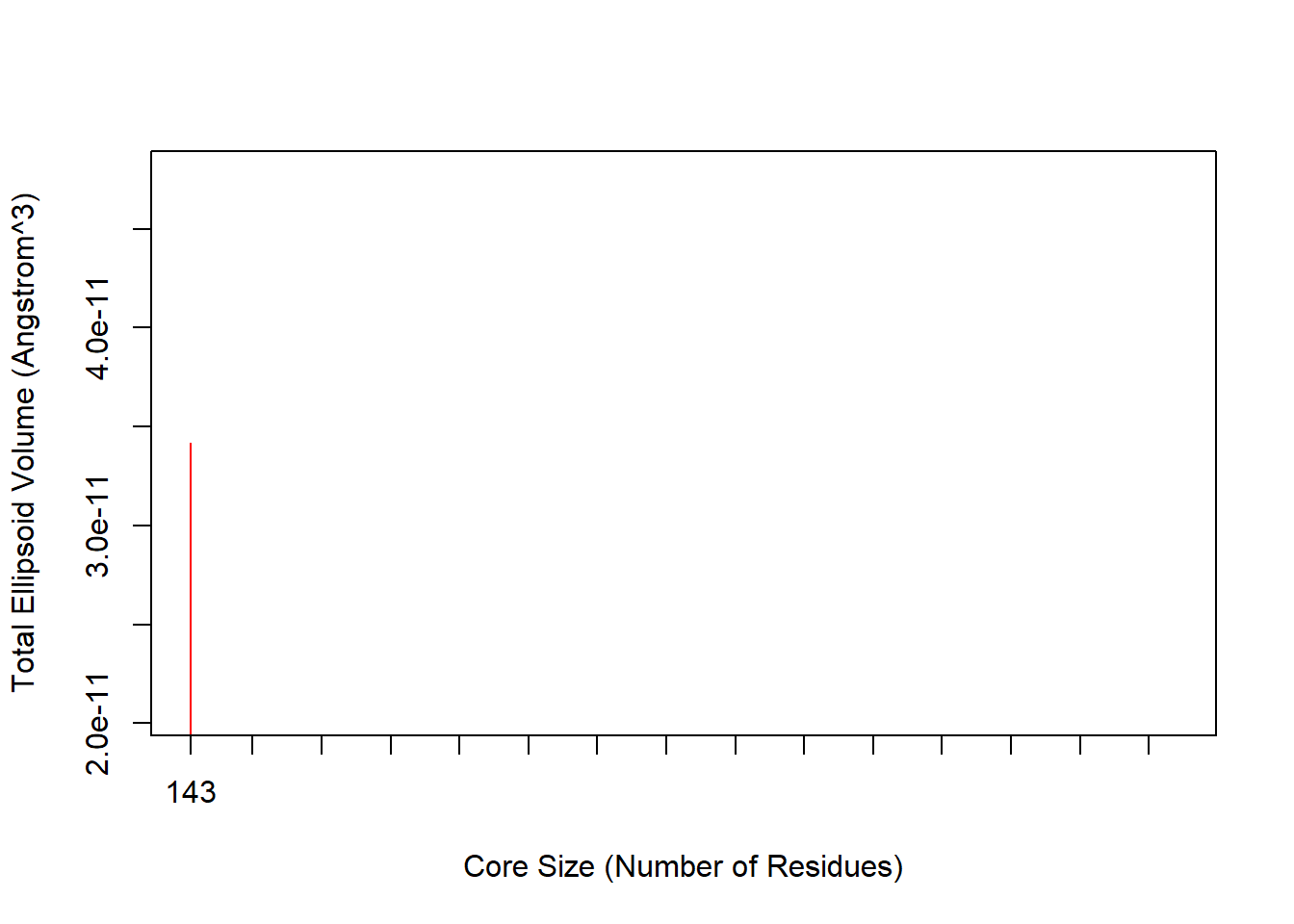
core.inds <- print(core, vol=1.0)# 144 positions (cumulative volume <= 1 Angstrom^3)
start end length
1 1 144 144xyz <- pdbfit( pdbs, core.inds, outpath = 'output/quick_fit.pdb' )
rd <- rmsd(xyz)Warning in rmsd(xyz): No indices provided, using the 144 non NA positionshist(rd, breaks=40, xlab="RMSD (Å)", main="Histogram of RMSD")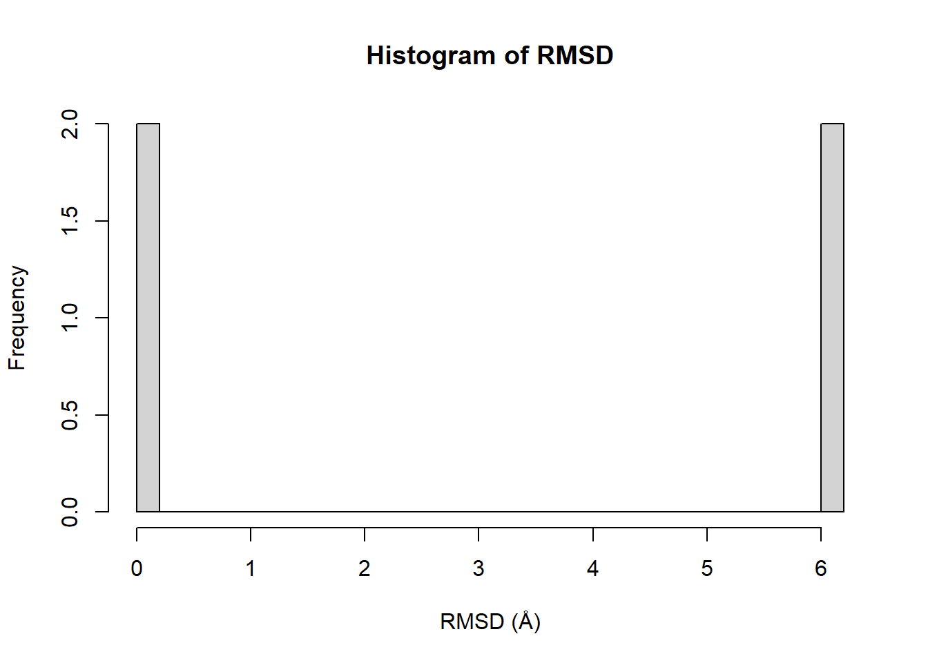
gaps.xyz2 <- gap.inspect(pdbs$xyz[c(1,2), ])
a.xyz <- pdbs$xyz[1, gaps.xyz2$f.inds]
b.xyz <- pdbs$xyz[2, gaps.xyz2$f.inds]
a <- torsion.xyz(a.xyz, atm.inc=1)
b <- torsion.xyz(b.xyz, atm.inc=1)
d.ab <- wrap.tor(a-b)
d.ab[is.na(d.ab)] <- 0
plot.bio3d(abs(d.ab), typ="h", xlab="Residue No.",
           ylab = "Difference Angle")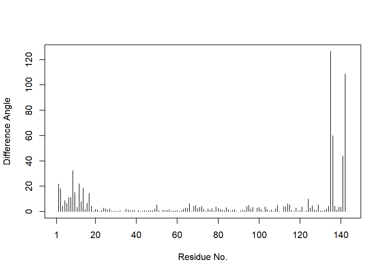
MUCH better.
a <- dm.xyz(a.xyz)
b <- dm.xyz(b.xyz)

plot.dmat( (a - b), nlevels=10, grid.col="gray", xlab="1tag", ylab="1tnd")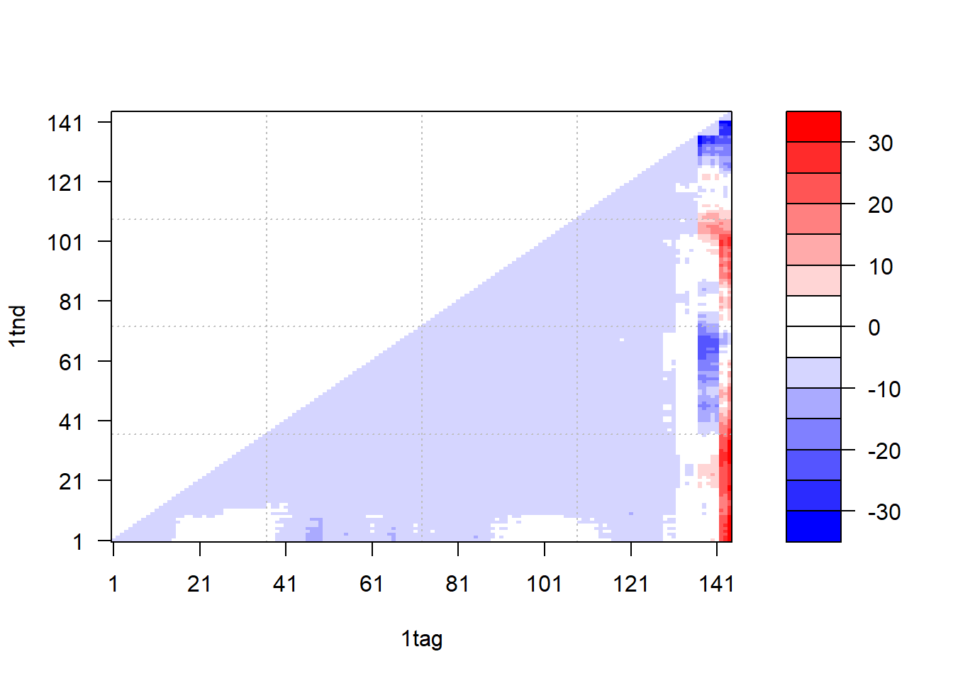
gaps.pos <- gap.inspect(pdbs$xyz)
pc.xray <- pca.xyz(xyz[, gaps.pos$f.inds])
pc.xray
Call:
  pca.xyz(xyz = xyz[, gaps.pos$f.inds])

Class:
  pca

Number of eigenvalues:
  432

        Eigenvalue Variance Cumulative
   PC 1   2619.076      100        100
   PC 2      0.000        0        100
   PC 3      0.000        0        100
   PC 4      0.000        0        100
   PC 5      0.000        0        100
   PC 6      0.000        0        100

   (Obtained from 2 conformers with 432 xyz input values).

+ attr: L, U, z, au, sdev, mean, call
plot(pc.xray)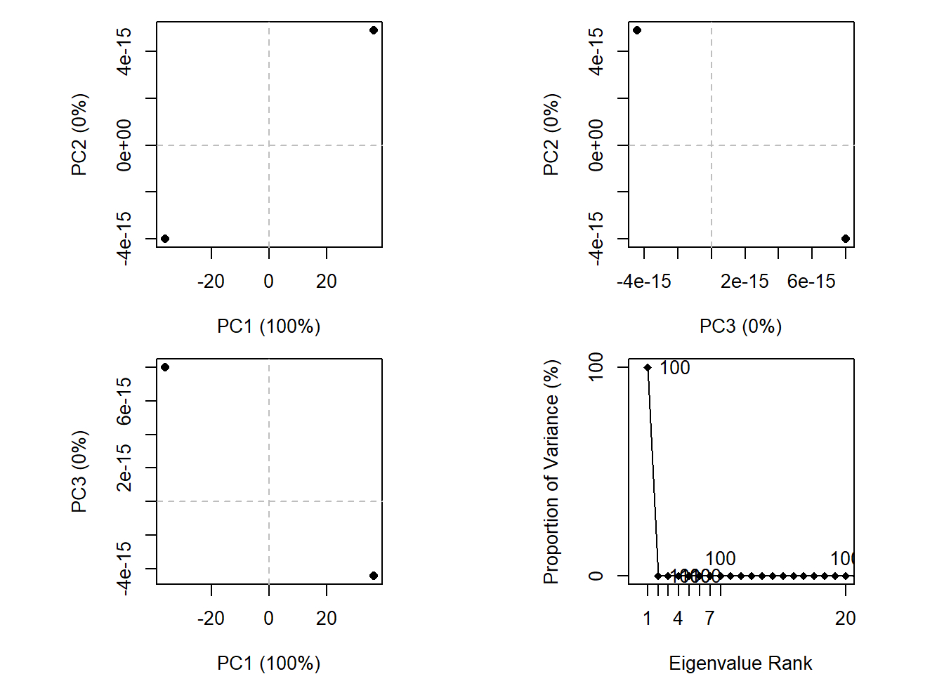
OK cool - now we can align all proteins and make proper plots!
sessionInfo()R version 4.1.0 (2021-05-18)
Platform: x86_64-w64-mingw32/x64 (64-bit)
Running under: Windows 10 x64 (build 19042)
Matrix products: default
locale:
[1] LC_COLLATE=English_Australia.1252 LC_CTYPE=English_Australia.1252
[3] LC_MONETARY=English_Australia.1252 LC_NUMERIC=C
[5] LC_TIME=English_Australia.1252
attached base packages:
[1] stats graphics grDevices utils datasets methods base
other attached packages:
[1] r3dmol_0.1.2 bio3d_2.4-3 workflowr_1.6.2
loaded via a namespace (and not attached):
[1] xfun_0.27 bslib_0.3.1 vctrs_0.3.8
[4] htmltools_0.5.2 stats4_4.1.0 yaml_2.2.1
[7] utf8_1.2.2 rlang_0.4.12 jquerylib_0.1.4
[10] later_1.3.0 pillar_1.6.4 glue_1.6.2
[13] BiocGenerics_0.38.0 GenomeInfoDbData_1.2.6 lifecycle_1.0.1
[16] stringr_1.4.0 zlibbioc_1.38.0 Biostrings_2.60.2
[19] htmlwidgets_1.5.4 evaluate_0.14 knitr_1.36
[22] IRanges_2.26.0 fastmap_1.1.0 httpuv_1.6.3
[25] GenomeInfoDb_1.28.4 parallel_4.1.0 fansi_0.5.0
[28] highr_0.9 msa_1.24.0 Rcpp_1.0.7
[31] xtable_1.8-4 promises_1.2.0.1 S4Vectors_0.30.2
[34] jsonlite_1.7.2 XVector_0.32.0 mime_0.12
[37] fs_1.5.0 digest_0.6.28 stringi_1.7.5
[40] shiny_1.7.1 grid_4.1.0 rprojroot_2.0.2
[43] tools_4.1.0 bitops_1.0-7 magrittr_2.0.1
[46] sass_0.4.0 RCurl_1.98-1.5 tibble_3.1.5
[49] crayon_1.4.1 whisker_0.4 pkgconfig_2.0.3
[52] ellipsis_0.3.2 rmarkdown_2.11 R6_2.5.1
[55] git2r_0.28.0 compiler_4.1.0