Visualising MSAs
Philipp Bayer
10 March 2022
Last updated: 2022-04-27
Checks: 7 0
Knit directory:
Amphibolis_Posidonia_Comparison/
This reproducible R Markdown analysis was created with workflowr (version 1.6.2). The Checks tab describes the reproducibility checks that were applied when the results were created. The Past versions tab lists the development history.
Great! Since the R Markdown file has been committed to the Git repository, you know the exact version of the code that produced these results.
Great job! The global environment was empty. Objects defined in the global environment can affect the analysis in your R Markdown file in unknown ways. For reproduciblity it’s best to always run the code in an empty environment.
The command set.seed(20210414) was run prior to running
the code in the R Markdown file. Setting a seed ensures that any results
that rely on randomness, e.g. subsampling or permutations, are
reproducible.
Great job! Recording the operating system, R version, and package versions is critical for reproducibility.
Nice! There were no cached chunks for this analysis, so you can be confident that you successfully produced the results during this run.
Great job! Using relative paths to the files within your workflowr project makes it easier to run your code on other machines.
Great! You are using Git for version control. Tracking code development and connecting the code version to the results is critical for reproducibility.
The results in this page were generated with repository version 0d3354b. See the Past versions tab to see a history of the changes made to the R Markdown and HTML files.
Note that you need to be careful to ensure that all relevant files for
the analysis have been committed to Git prior to generating the results
(you can use wflow_publish or
wflow_git_commit). workflowr only checks the R Markdown
file, but you know if there are other scripts or data files that it
depends on. Below is the status of the Git repository when the results
were generated:
Ignored files:
    Ignored:    .Rhistory
    Ignored:    .Rproj.user/
    Ignored:    analysis/OTT.nb.html
    Ignored:    analysis/plotRgenes.nb.html

Untracked files:
    Untracked:  output/EIN3_better_phylogeny.png
    Untracked:  output/SOS3_better_phylogeny.png

Unstaged changes:
    Modified:   output/SOS3_phylogeny.png
Note that any generated files, e.g. HTML, png, CSS, etc., are not included in this status report because it is ok for generated content to have uncommitted changes.
These are the previous versions of the repository in which changes were
made to the R Markdown (analysis/MSA.Rmd) and HTML
(docs/MSA.html) files. If you’ve configured a remote Git
repository (see ?wflow_git_remote), click on the hyperlinks
in the table below to view the files as they were in that past version.
| File | Version | Author | Date | Message |
|---|---|---|---|---|
| Rmd | 0d3354b | Philipp Bayer | 2022-04-27 | Better phylogenies |
| html | 3c7f16f | Philipp Bayer | 2022-03-23 | Build site. |
| Rmd | 9093bee | Philipp Bayer | 2022-03-23 | workflowr::wflow_publish(files = "analysis/MSA.Rmd") |
| html | c176104 | Philipp Bayer | 2022-03-16 | Build site. |
| Rmd | a02475f | Philipp Bayer | 2022-03-16 | fix MSA code to be nicer |
| html | 61333e0 | Philipp Bayer | 2022-03-11 | Build site. |
| Rmd | e9128f4 | Philipp Bayer | 2022-03-11 | fix MSA |
| html | 56d032a | Philipp Bayer | 2022-03-11 | Build site. |
| Rmd | 76a65cd | Philipp Bayer | 2022-03-11 | finalised MSA! |
| html | a994174 | Philipp Bayer | 2022-03-10 | Build site. |
| Rmd | e57f6d8 | Philipp Bayer | 2022-03-10 | Fix one label! |
| Rmd | ebd08f5 | Philipp Bayer | 2022-03-10 | Add missing files |
| html | ebd08f5 | Philipp Bayer | 2022-03-10 | Add missing files |
| html | 8886b0e | Philipp Bayer | 2022-03-10 | Build site. |
| Rmd | 02708fd | Philipp Bayer | 2022-03-10 | New: fancy MSAs!! |
I found some interesting gene clusters. Let’s look at them
library(tidyverse)
library(ggmsa)
library(Biostrings)
library(ape)
library(ggtree)
library(treeio)
knitr::opts_knit$set(root.dir = rprojroot::find_rstudio_root_file())
ggmsa('data/SOS3_OG0000189/OG0000189.RiceAraSeagrasses.aln.fasta', start = 221, end = 260, char_width = 0.5, seq_name = T) + geom_seqlogo() + geom_msaBar()Coordinate system already present. Adding new coordinate system, which will replace the existing one.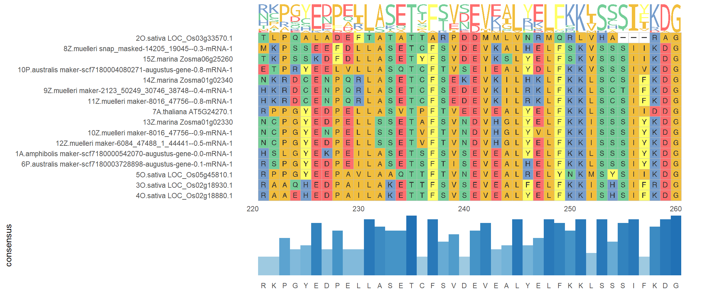
x <- readAAStringSet('data/SOS3_OG0000189/OG0000189.RiceAraSeagrasses.aln.fasta')
d <- as.dist(stringDist(x, method = "hamming")/width(x)[1])
tree <- bionj(d)
p <- ggtree(tree) + geom_tiplab()
ggtree(tree) + geom_tiplab()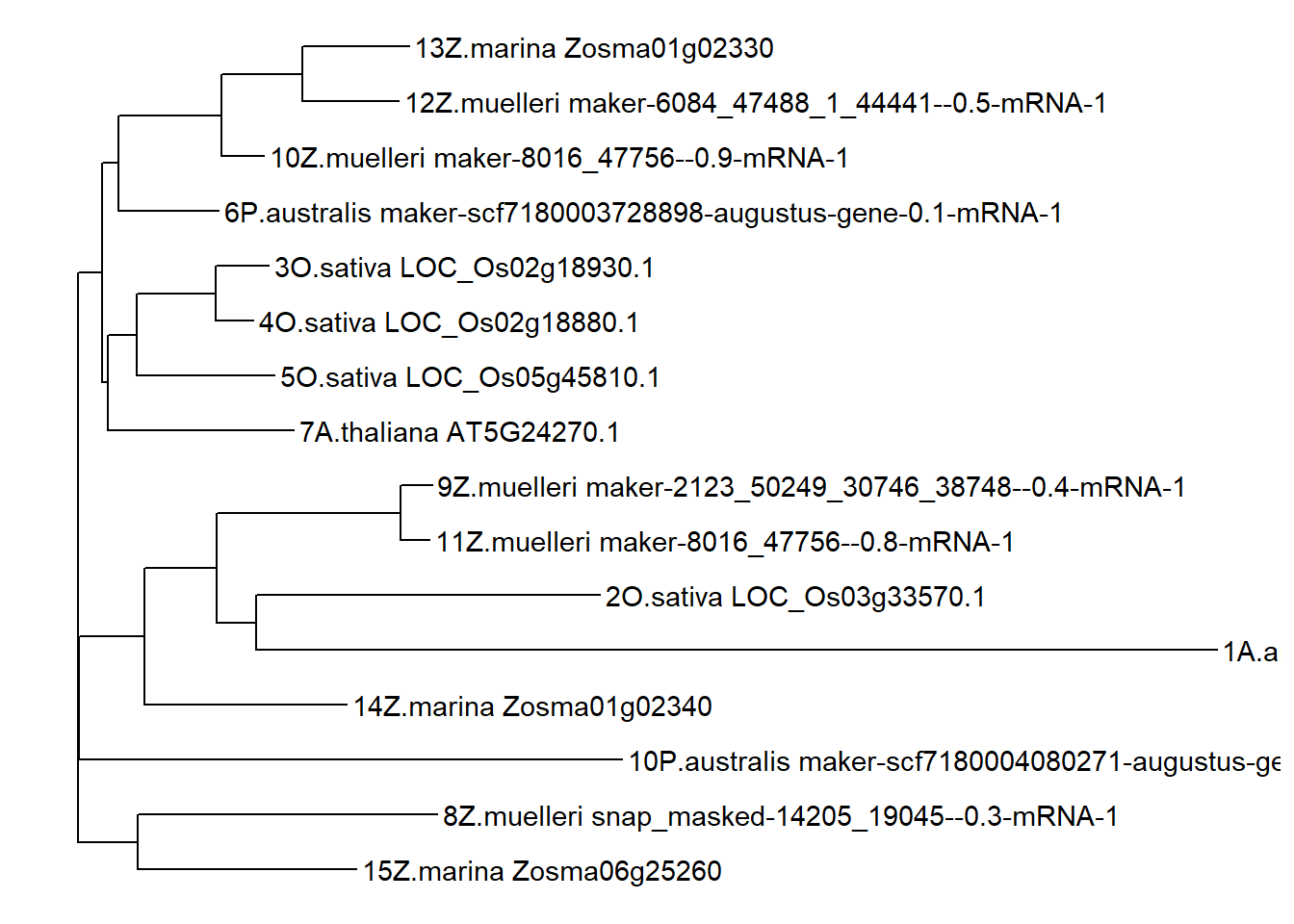
data <- tidy_msa('data/SOS3_OG0000189/OG0000189.RiceAraSeagrasses.aln.fasta', 221, 300)
p + geom_facet(geom = geom_msa, data = data,  panel = 'Multiple Sequence Alignment (221-300AA)',
               font = NULL, color = "Clustal", by_conversation= TRUE) +
    xlim_tree(1)
Warning: Unknown or uninitialised column: `name`.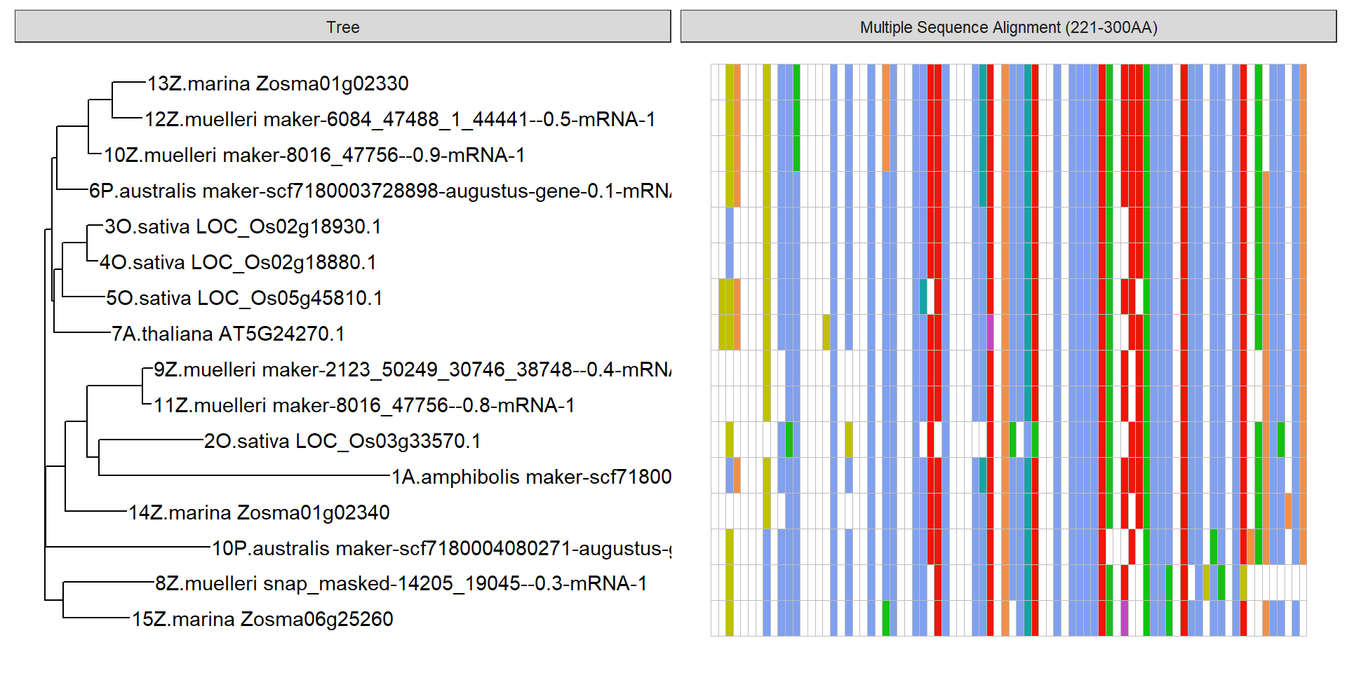
Let’s use a RAXML made tree
Commands run, after I shortened protein IDs manually. I pulled out the rice/Arabidopsis/seagrass proteins manually from the OG0000189.fa Orthofinder produced, and shortened their names so they fit into Phylip format.
muscle -in OG0000189.RiceAraSeagrasses.fa -out OG0000189.RiceAraSeagrasses.phy -phyi
raxmlHPC -p12345 -m PROTGAMMAAUTO -s OG0000189.RiceAraSeagrasses.phy -n AUTO
treestring <- '((3O.sativa:0.11386470583955717040,4O.sativa:0.03615896391829190315):0.07379737996482453599,(5O.sativa:0.33751444720146173140,((7A.thalian:0.45696796911334131019,((8Z.mueller:0.33996861614583556710,15Z.marina:0.16088168380872580610):0.31923212677234219514,10P.austra:0.57486248434538900209):0.22324965676023655892):0.10039129162924786964,((13Z.marina:0.11346816437532522559,(12Z.muelle:0.00973855109814669891,10Z.muelle:0.02645894329604922546):0.09840311662577182206):0.35332170475064506032,((14Z.marina:0.12821969530885793387,(9Z.mueller:0.06883167458475099310,11Z.muelle:0.02355162378347611801):0.15839770535961147924):0.63099939044074537797,(1A.amphibo:0.53760770644490452064,6P.austral:0.07001018412366488697):0.08839123570898912985):0.05074368132159561007):0.09141392275039983417):0.12967268161775510893):0.11320488597472283532,2O.sativa:1.70657194075952300949):0.0;'
plot(ape::read.tree(text=treestring))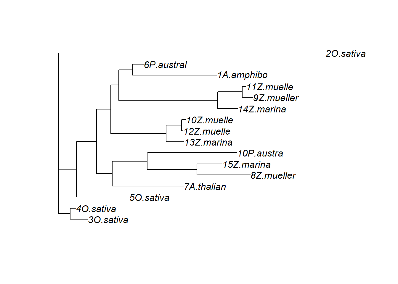
p2 <- ggtree(ape::read.tree(text=treestring)) + geom_tiplab()
p2
That’s very different from the above dendrogram!
data2 <- data %>% mutate(name = str_sub(name, 1, 10),
                         name = str_trim(name))
p2 + geom_facet(geom = geom_msa, data = data2,  panel = 'Multiple Sequence Alignment (221-260AA)',
               font = NULL, color = "Clustal") +
    xlim_tree(2)
Warning: Unknown or uninitialised column: `name`.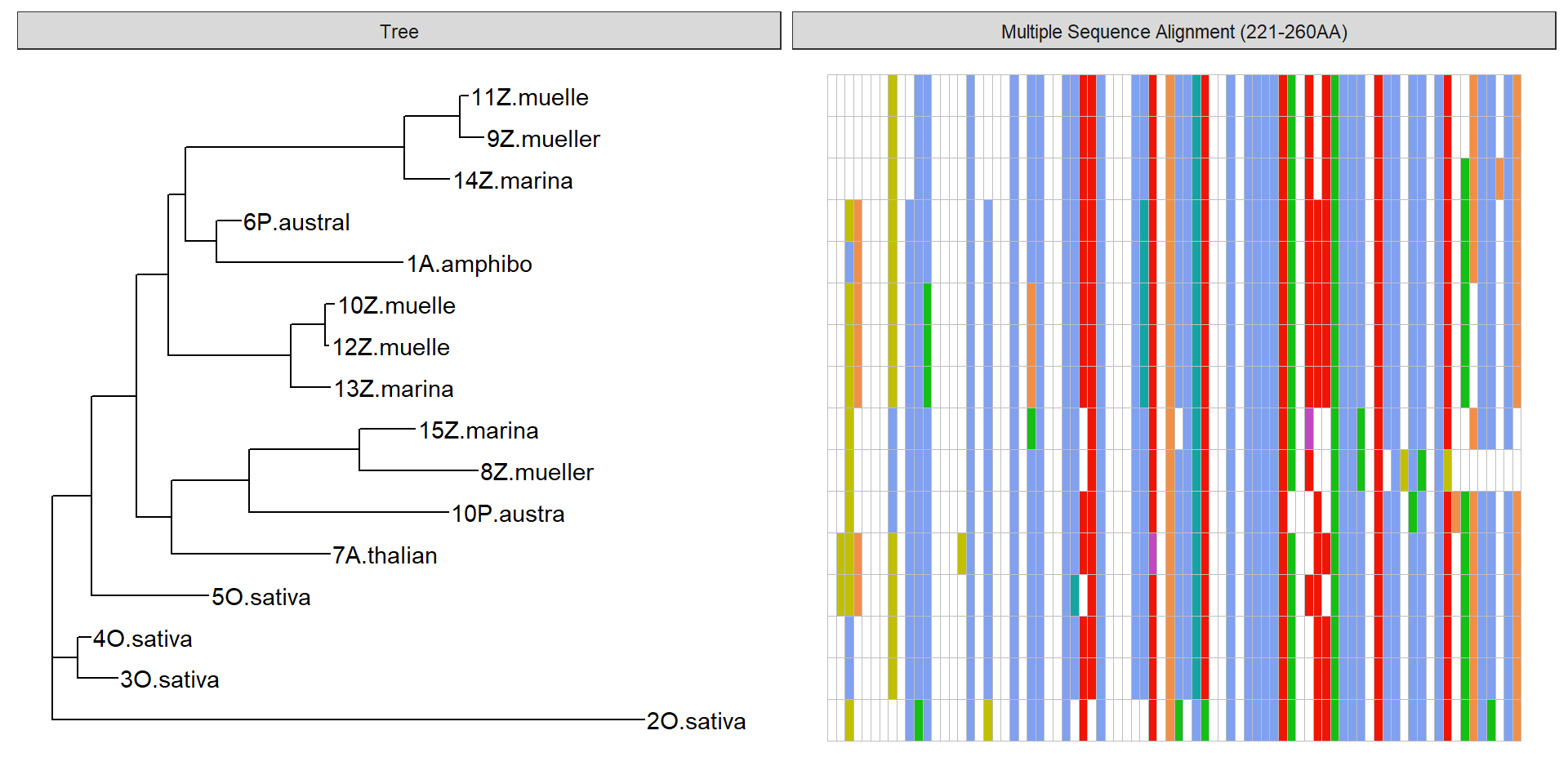
Good! I used blastp with Swissprot to see whether I could get ‘official’ gene names for some of these, especially the O. sativa. I uploaded the fasta in data/OG000189.fa to blastp/swissprot, and pulled out new names where available.
Hits are to: A. thaliana Calcineurin B-like protein 4 (CBL4, Alternative name: SOS3) O. sativa Calcineurin B-like protein 8 (CBL8) O. sativa Calcineurin B-like protein 4 (CBL4)
Let’s rename the tree and the MSA data table using
rename_taxa
trees <- ape::read.tree(text=treestring)

rename_df <- tibble::tribble(
                       ~old,        ~new,
                "3O.sativa",    "OsCBL8",
                "4O.sativa",  "OsCBL7.1",
                "5O.sativa",    "OsCBL4",
               "7A.thalian",    "AtSOS3",
               "8Z.mueller",   "ZmuSOS3",
               "15Z.marina",   "ZmaSOS3",
               "10P.austra",    "PaSOS3",
               "13Z.marina", "ZmaSOS3.2",
               "12Z.muelle", "ZmuSOS3.2",
               "10Z.muelle", "ZmuSOS3.3",
               "14Z.marina", "ZmaSOS3.2",
               "9Z.mueller", "ZmuSOS3.4",
               "11Z.muelle", "ZmuSOS3.5",
               "1A.amphibo",    "AaSOS3",
               "6P.austral",  "PaSOS3.2",
                "2O.sativa",  "OsCBL7.2"
               )


trees <- rename_taxa(trees, rename_df, old, new)
p3 <- ggtree(trees) + geom_tiplab(fontface='italic')

p3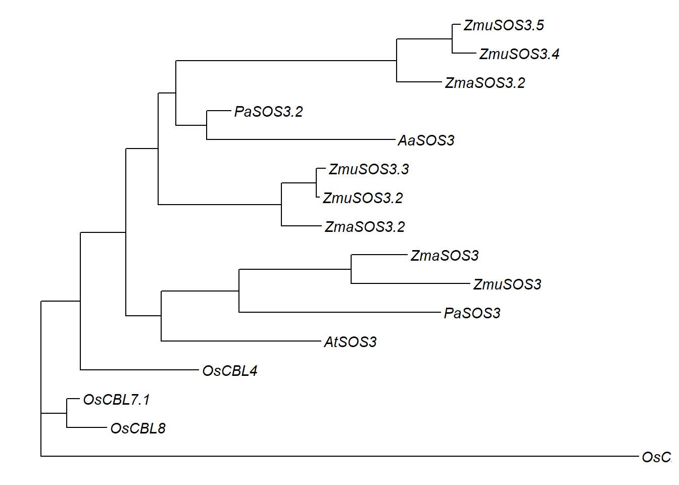
#str_replace_all takes a named vector
replace_vector <- rename_df$new
names(replace_vector) <- rename_df$old
data2 <- data2 %>% mutate(name = str_replace_all(name, replace_vector))
final_p <- p3 + geom_facet(geom = geom_msa, data = data2, panel = 'Multiple Sequence Alignment (221-260AA)',
font = NULL, color = "Chemistry_AA") +
xlim_tree(2)Warning: Unknown or uninitialised column: `name`.final_p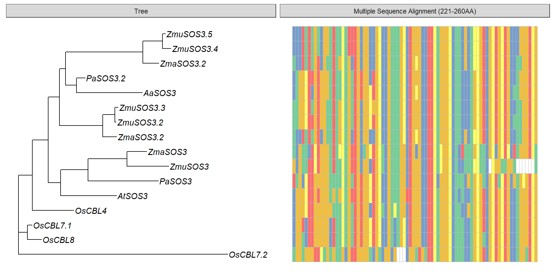
cowplot::save_plot(final_p, filename = 'output/SOS3_phylogeny.png', base_width=10)“However, apparent photosynthesis is still maintained at a salinity 15% that of normal seawater and at temperatures of 3 and 30°C, consistent with the ecological role of Z. muelleri as an intertidal species.” https://www.sciencedirect.com/science/article/abs/pii/0304377085900634
Now let’s also add support values.
I ran this based on Using RAxML-NG in Practice
Phylogeny for the SOS3 cluster
 # to get best model
modeltest-ng -i OG0000189.RiceAraSeagrasses.aln.fasta -t ml -d aa -p 8

 # to get fixed fasta
raxml-ng --msa OG0000189.RiceAraSeagrasses.aln.fasta --model JTT-DCMUT+G4 --check

# to make a regular tree
raxml-ng --msa OG0000189.RiceAraSeagrasses.aln.fasta.raxml.reduced.phy --model JTT-DCMUT+G4 --prefix T3 --threads 2 --seed 2

# make 200 bootstrap trees, does not converge
raxml-ng --msa OG0000189.RiceAraSeagrasses.aln.fasta.raxml.reduced.phy --model JTT-DCMUT+G4 --prefix T8 --threads 8 --seed 2 --bootstrap --bs-trees 200

# make another 400  with different seed
raxml-ng --msa OG0000189.RiceAraSeagrasses.aln.fasta.raxml.reduced.phy --model JTT-DCMUT+G4 --prefix T11 --threads 8 --seed 333 --bootstrap --bs-trees 400

# check whether they converge with <3% WRF cutoff
raxml-ng --bsconverge --bs-trees allbootstraps --prefix T12 --seed 2 --threads 1 --bs-cutoff 0.03


# to make the final trees with bootstrap values

cat T8.raxml.bootstraps T11.raxml.bootstraps > allbootstraps

raxml-ng --support --tree T3.raxml.bestTree --bs-trees allbootstraps --prefix T13

#yes, after 550 - close one!

# let's make another 400 so we can have a nice 1000 bootstraps - different seed again!

raxml-ng --msa OG0000189.RiceAraSeagrasses.aln.fasta.raxml.reduced.phy --model JTT-DCMUT+G4 --prefix T14 --threads 8 --seed 1234 --bs-trees 400  --bootstrap

cat T8.raxml.bootstraps T11.raxml.bootstraps T14.raxml.bootstraps > allbootstraps
raxml-ng --support --tree T3.raxml.bestTree --bs-trees allbootstraps --prefix T15
newtree <- '((((((12Z.muelleri_maker-6084_47488_1_44441--0.5-mRNA-1:0.009685,10Z.muelleri_maker-8016_47756--0.9-mRNA-1:0.026505)99:0.098293,13Z.marina_Zosma01g02330:0.113268)99:0.354433,(((11Z.muelleri_maker-8016_47756--0.8-mRNA-1:0.023273,9Z.muelleri_maker-2123_50249_30746_38748--0.4-mRNA-1:0.068317)99:0.153634,14Z.marina_Zosma01g02340:0.129762)100:0.616637,(1A.amphibolis_maker-scf7180000542070-augustus-gene-0.0-mRNA-1:0.518908,6P.australis_maker-scf7180003728898-augustus-gene-0.1-mRNA-1:0.074916)72:0.082830)22:0.047398)31:0.080205,((2O.sativa_LOC_Os03g33570.1:1.647537,(3O.sativa_LOC_Os02g18930.1:0.113637,4O.sativa_LOC_Os02g18880.1:0.035299)53:0.061341)66:0.111396,5O.sativa_LOC_Os05g45810.1:0.344545)75:0.137407)42:0.100482,7A.thaliana_AT5G24270.1:0.448151)83:0.209634,(15Z.marina_Zosma06g25260:0.152988,8Z.muelleri_snap_masked-14205_19045--0.3-mRNA-1:0.336420)100:0.314204,10P.australis_maker-scf7180004080271-augustus-gene-0.8-mRNA-1:0.580458)83:0.0;'

tree3 <- ape::read.tree(text=newtree, branch.label='support')

p3 <- ggtree(tree3) + geom_tiplab()
p3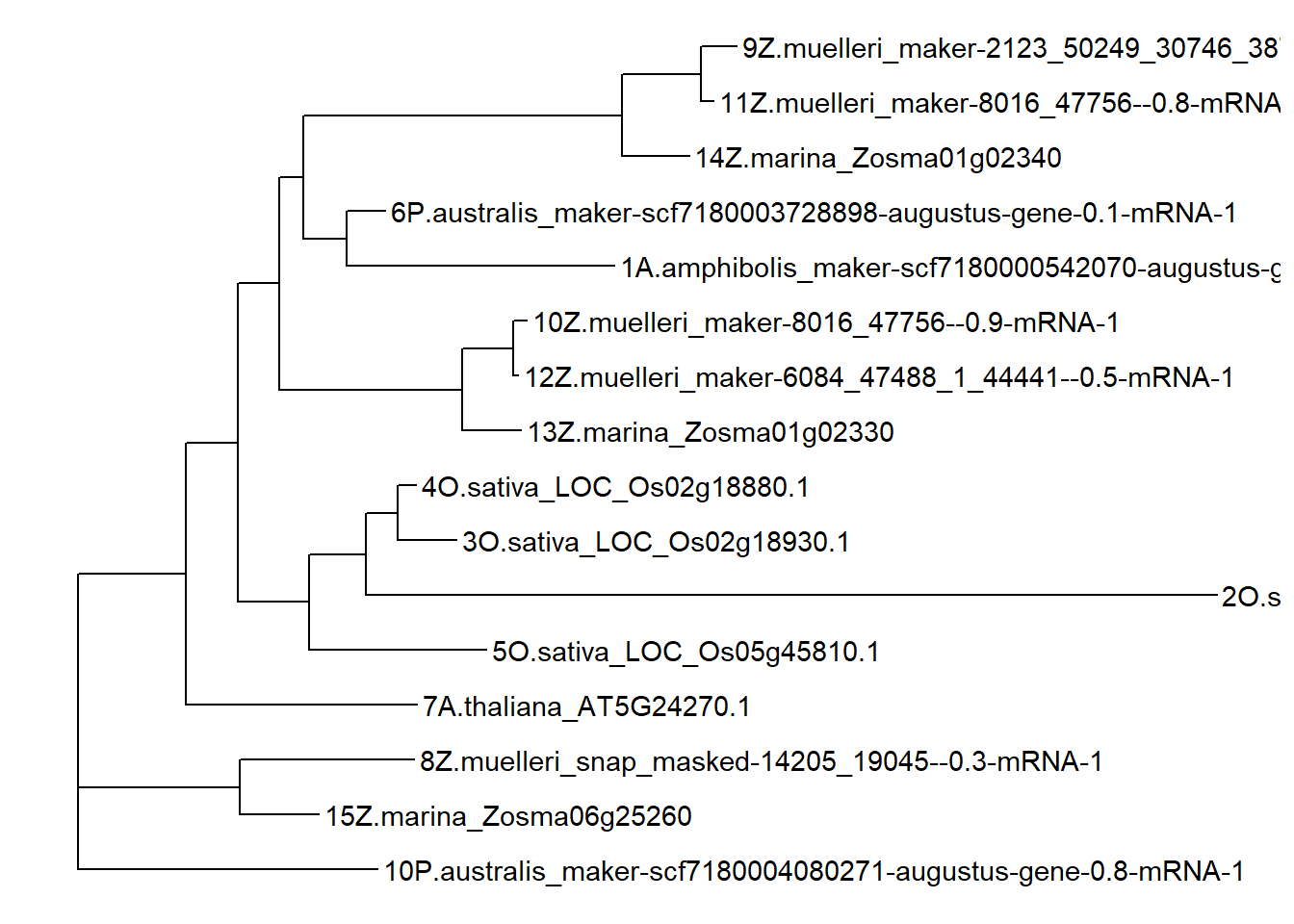
OK the nodes are now named differently due to raxml-ng, time to fix again
old_names <- tree3$tip.label

# [1] "3O.sativa"  "4O.sativa"  "5O.sativa"  "7A.thalian" "8Z.mueller" "15Z.marina" "10P.austra" "13Z.marina"
# [9] "12Z.muelle" "10Z.muelle" "14Z.marina" "9Z.mueller" "11Z.muelle" "1A.amphibo" "6P.austral" "2O.sativa"
#new_names  <- c( 'OsCBL8', 'OsCBL7.1', 'OsCBL4', 'AtSOS3', 'ZmuSOS3', 'ZmaSOS3', 'PaSOS3', 'ZmaSOS3.2',
#                 'ZmuSOS3.2', 'ZmuSOS3.3', 'ZmaSOS3.3', 'ZmuSOS3.2', 'ZmuSOS3.4', 'AaSOS3', 'PaSOS3.2', 'OsCBL7.2')
new_names  <- c('ZmuSOS3.2', 'ZmuSOS3.3', 'ZmaSOS3.2', 'ZmuSOS3.4', 'ZmuSOS3.5', 'ZmaSOS3.3','AaSOS3',
                'PaSOS3.2', 'OsCBL7.2', 'OsCBL8', 'OsCBL7.1', 'OsCBL4', 'AtSOS3', 'ZmaSOS3', 'ZmuSOS3', 'PaSOS3')
rename_df <- data.frame(old = old_names, new = new_names)


tree3 <- rename_taxa(tree3, rename_df, old, new)
p3 <- ggtree(tree3) + geom_tiplab(fontface='italic')
p3 <- p3 + geom_nodelab(aes(subset=label>80), label='*')
p3+ ggplot2::xlim(0,2.5)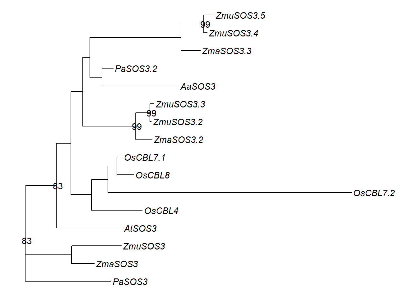
muhtree <- ggtree(tree3)
my_data <- muhtree$data
my_data <- my_data %>% mutate(support = replace_na(as.numeric(label), 0))
Warning in replace_na(as.numeric(label), 0): NAs introduced by coercionroot <- rootnode(tree3)
good_p <- ggtree(tree3) %<+% my_data +
geom_tiplab(fontface = 'italic') +
geom_point2(aes(
subset = !isTip & node != root,
fill = cut(support, c(-1, 70, 90, 100))
),
shape = 21,
size = 4) +
scale_fill_manual(
values = c('#d95f02', '#7570b3', '#1b9e77'),
labels = expression(BP < 70, 70 <= BP * " < 90", BP >= 90),
name = 'Bootstrap Percentage',
breaks = c('(-1,70]', '(70,90]', '(90,100]')
) +
ggplot2::xlim(0, 2.5) +
theme_tree(legend.position = 'bottom')
good_p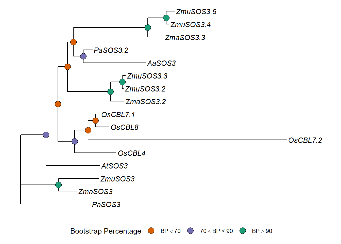
cowplot::save_plot(good_p, filename = 'output/SOS3_better_phylogeny.png')replace_vector <- new_names
names(replace_vector) <- old_names
data <- tidy_msa('data/SOS3_OG0000189/OG0000189.RiceAraSeagrasses.aln.fasta', 221, 260)
data3 <- data %>% mutate(name = str_replace(name, ' ', '_'),
name = str_replace_all(name, replace_vector))
p3 + geom_facet(geom = geom_msa, data = data3, panel = 'Multiple Sequence Alignment (221-260AA)',
font = NULL, color = "Chemistry_AA") +
xlim_tree(3)Warning: Unknown or uninitialised column: `name`.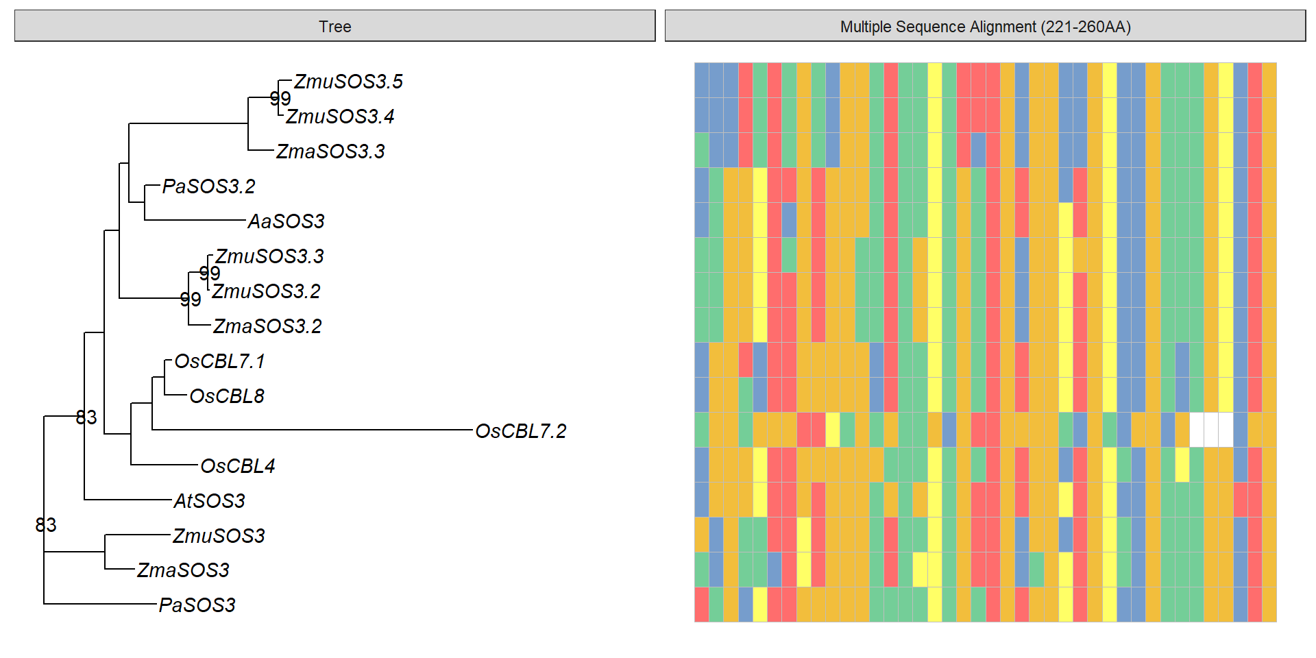
msaplot(p3, 'data/SOS3_OG0000189/OG0000189.RiceAraSeagrasses.aln.NamesFixed.fasta',
        offset = 0.5) + theme(legend.position='none')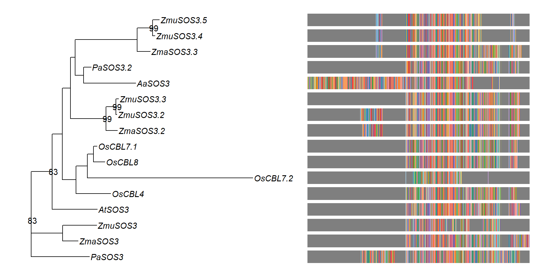
Phylogeny for the EIN3 cluster
First, to align the sequences again:
modeltest-ng reports JTT+I+G4+F

raxml-ng --msa OG0000629.RiceAraSeagrasses.aln.fa --model JTT+I+G4+F


 # to get fixed fasta - all good!!
raxml-ng --msa OG0000629.RiceAraSeagrasses.aln.fa --model JTT+I+G4+F --check

# to make a regular tree
raxml-ng --msa OG0000629.RiceAraSeagrasses.aln.fa --model JTT+I+G4+F --prefix T3 --threads 2 --seed 2

# make 1000 bootstrap trees
raxml-ng --msa OG0000629.RiceAraSeagrasses.aln.fa --model JTT+I+G4+F --prefix T8 --threads 16 --seed 2 --bootstrap --bs-trees 1000

# check whether they converge with <3% WRF cutoff
raxml-ng --bsconverge --bs-trees T8.raxml.bootstraps --prefix T12 --seed 2 --threads 1 --bs-cutoff 0.03

# it actually converged with 50 trees. haha.

# to make the final trees with bootstrap values

raxml-ng --support --tree T3.raxml.bestTree --bs-trees allbootstraps --prefix T13
There we go:
tree3 <- ape::read.tree(text='(((LOC_Os07g48630.1:0.641123,(LOC_Os03g20780.1:0.007239,LOC_Os03g20790.1:0.001048)100:0.214718)100:0.418001,(((Zosma02g24210:0.119273,(maker-1834_92013--0.52-mRNA-1:0.074816,augustus_masked-5412_21708--0.0-mRNA-1:0.082668)97:0.073791)100:0.640955,augustus_masked-scf7180003860583-processed-gene-0.3-mRNA-1:0.182720)89:0.114788,(maker-3356_51779--0.18-mRNA-1:0.661393,Zosma01g42670:0.320772)100:0.468870)67:0.098845)100:0.660268,AT3G20770.1:0.149857,AT2G27050.1:0.250165)100:0.0;', branch.label='support')

rename_df <- tibble::tribble(
                                                       ~old,        ~new,
                                         "LOC_Os07g48630.1",    "OsEIL2",
                                         "LOC_Os03g20780.1",    "OsEIL1",
                                         "LOC_Os03g20790.1",  "OsEIL1.2",
                                            "Zosma02g24210", "ZmaEIN3.1",
                            "maker-1834_92013--0.52-mRNA-1", "ZmuEIN3.1",
                   "augustus_masked-5412_21708--0.0-mRNA-1", "ZmuEIN3.2",
"augustus_masked-scf7180003860583-processed-gene-0.3-mRNA-1",   "PaEIN3",
                            "maker-3356_51779--0.18-mRNA-1", "ZmuEIN3.3",
                                            "Zosma01g42670", "ZmaEIN3.2",
                                              "AT3G20770.1",    "AtEIN3",
                                              "AT2G27050.1",    "AtEIL1"
               )

tree3 <- rename_taxa(tree3, rename_df, old, new)

p3 <-  ggtree(tree3) + geom_tiplab(fontface='italic')
p3 <- p3 + geom_nodelab()
p3 + xlim_tree(2.1)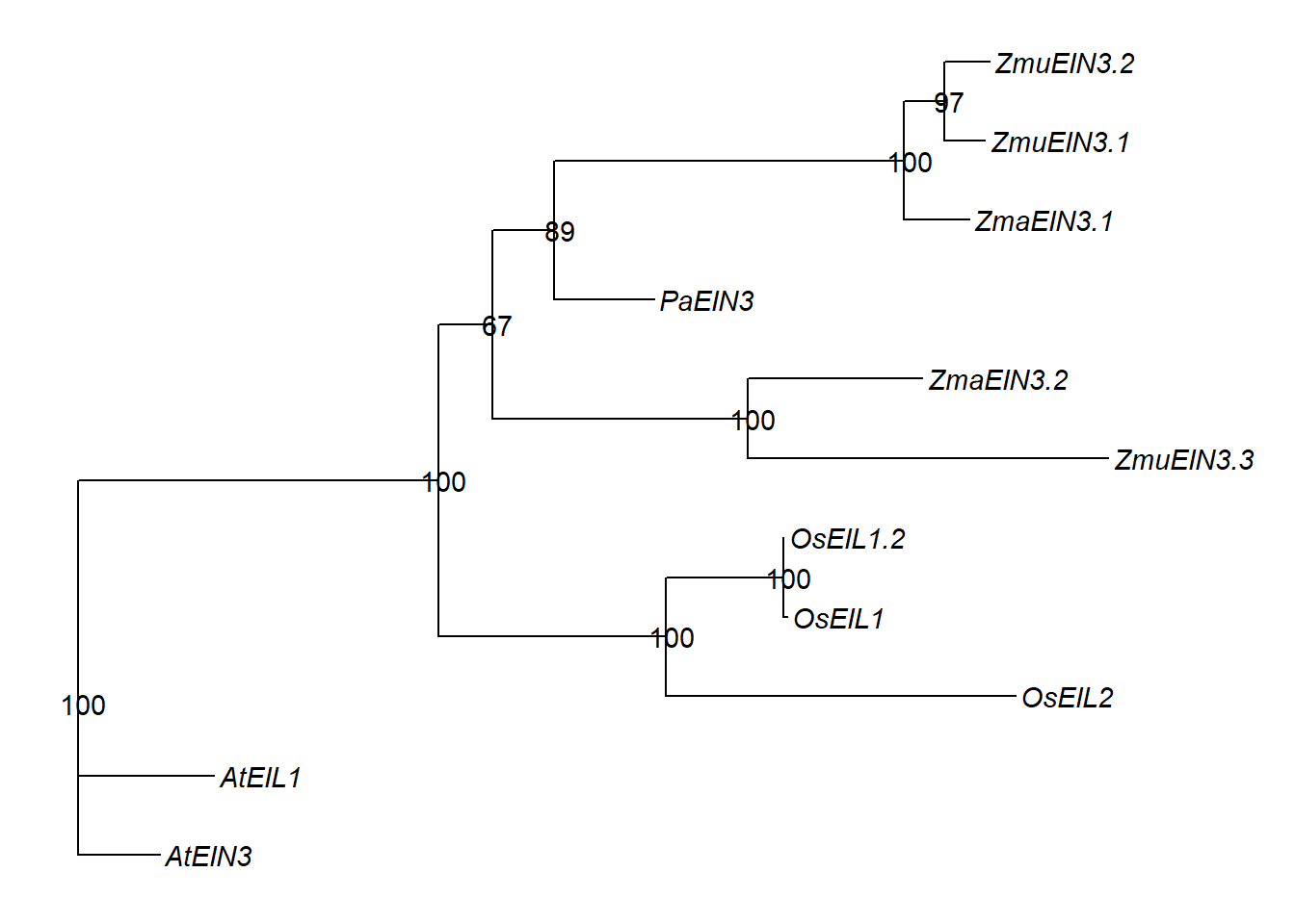
muhtree <- ggtree(tree3)
my_data <- muhtree$data
my_data <- my_data %>% mutate(support = replace_na(as.numeric(label), 0))
Warning in replace_na(as.numeric(label), 0): NAs introduced by coercionroot <- rootnode(tree3)
good_p <- ggtree(tree3) %<+% my_data +
geom_tiplab(fontface = 'italic') +
geom_point2(aes(
subset = !isTip & node != root,
fill = cut(support, c(-1, 70, 90, 100))
),
shape = 21,
size = 4) +
scale_fill_manual(
values = c('#d95f02', '#7570b3', '#1b9e77'),
labels = expression(BP < 70, 70 <= BP * " < 90", BP >= 90),
name = 'Bootstrap Percentage',
breaks = c('(-1,70]', '(70,90]', '(90,100]')
) +
ggplot2::xlim(0, 2.5) +
theme_tree(legend.position = 'bottom')
good_p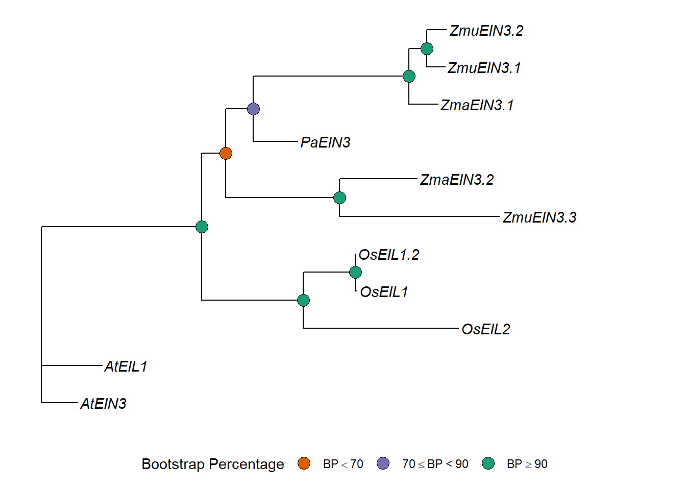
cowplot::save_plot(good_p, filename = 'output/EIN3_better_phylogeny.png')msaplot(p3, './data/EIN3_OG0000629/OG0000629.RiceAraSeagrasses.aln.NamesFixed.fa',
offset = 0.5) + theme(legend.position='none')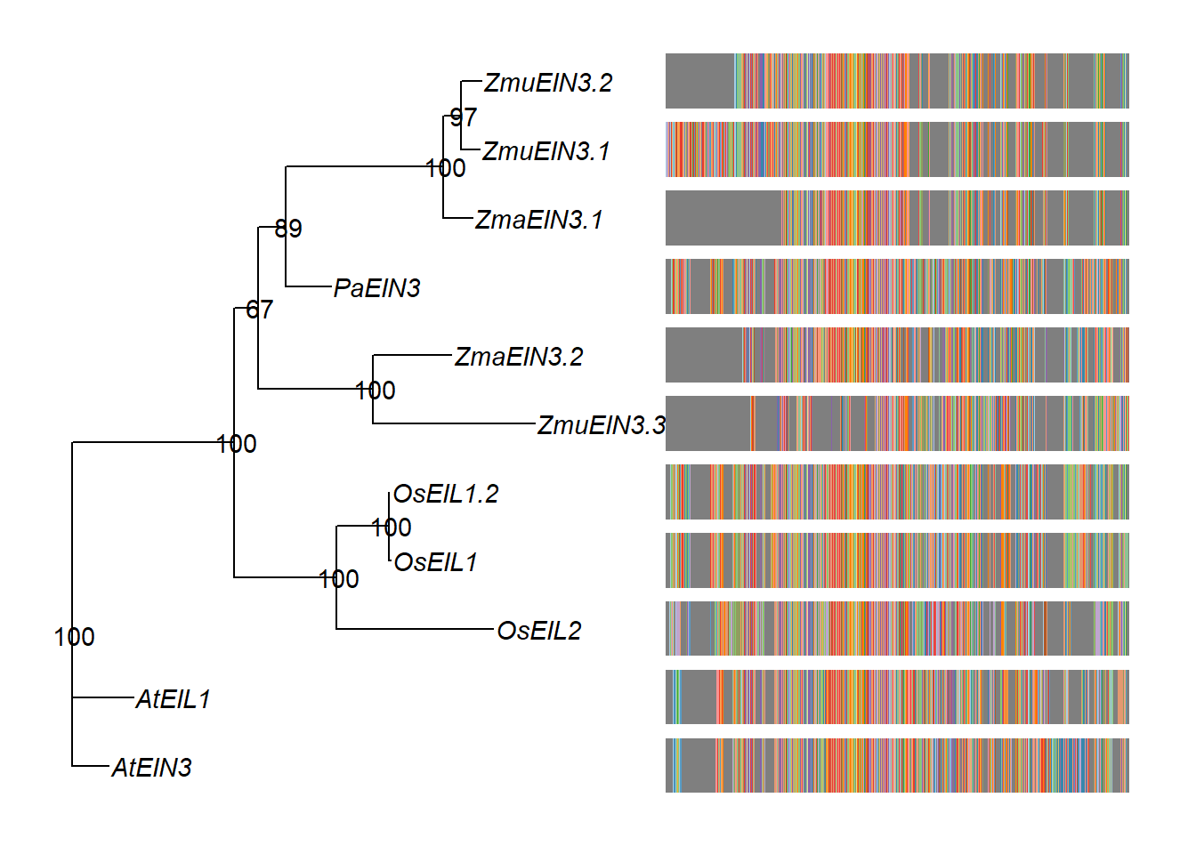
domains <- tibble::tribble(
~Gene, ~Pfam, ~Start, ~End, ~Evalue,
"Zosma01g42670", "PF04873", 3L, 246L, 2.9e-117,
"AT2G27050.1", "PF04873", 49L, 298L, 2.6e-130,
"LOC_Os03g20780.1", "PF04873", 78L, 332L, 1.4e-132,
"augustus_masked-scf7180003860583-processed-gene-0.3-mRNA-1", "PF04873", 76L, 325L, 1.9e-131,
"maker-1834_92013--0.52-mRNA-1", "PF04873", 136L, 408L, 2e-123,
"LOC_Os07g48630.1", "PF04873", 81L, 338L, 3.7e-129,
"AT3G20770.1", "PF04873", 49L, 296L, 4.8e-129,
"augustus_masked-5412_21708--0.0-mRNA-1", "PF04873", 16L, 285L, 2.2e-123,
"maker-3356_51779--0.18-mRNA-1", "PF04873", 85L, 125L, 2e-12,
"LOC_Os03g20790.1", "PF04873", 78L, 332L, 1.4e-132,
"Zosma02g24210", "PF04873", 1L, 206L, 1.9e-113
)
domains$length <- domains$End - domains$Start
replace_vector <- rename_df$new
names(replace_vector) <- rename_df$old
domains <- domains %>% mutate(Gene = str_replace_all(Gene, replace_vector))
domains# A tibble: 11 x 6
Gene Pfam Start End Evalue length
<chr> <chr> <int> <int> <dbl> <int>
1 ZmaEIN3.2 PF04873 3 246 2.9e-117 243
2 AtEIL1 PF04873 49 298 2.6e-130 249
3 OsEIL1 PF04873 78 332 1.4e-132 254
4 PaEIN3 PF04873 76 325 1.9e-131 249
5 ZmuEIN3.1 PF04873 136 408 2 e-123 272
6 OsEIL2 PF04873 81 338 3.7e-129 257
7 AtEIN3 PF04873 49 296 4.8e-129 247
8 ZmuEIN3.2 PF04873 16 285 2.2e-123 269
9 ZmuEIN3.3 PF04873 85 125 2 e- 12 40
10 OsEIL1.2 PF04873 78 332 1.4e-132 254
11 ZmaEIN3.1 PF04873 1 206 1.9e-113 205g <- domains %>% left_join(rename_df, by=c('Gene'='new')) %>% ggplot(aes(y = Gene, yend=Gene, x=Start, xend=End, color=Evalue)) + geom_segment(size=2) + theme_minimal() + xlab(expression(paste("Position of ", italic("EIN3"))))
g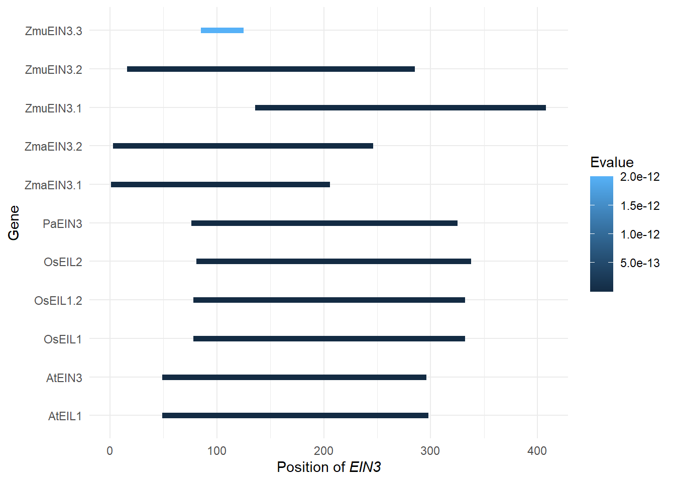
library(aplot)Warning: package 'aplot' was built under R version 4.1.2g <- g + theme(axis.title.y=element_blank(),
axis.text.y = element_blank(),
legend.position='none')
g %>% insert_left(p3, width=2.5)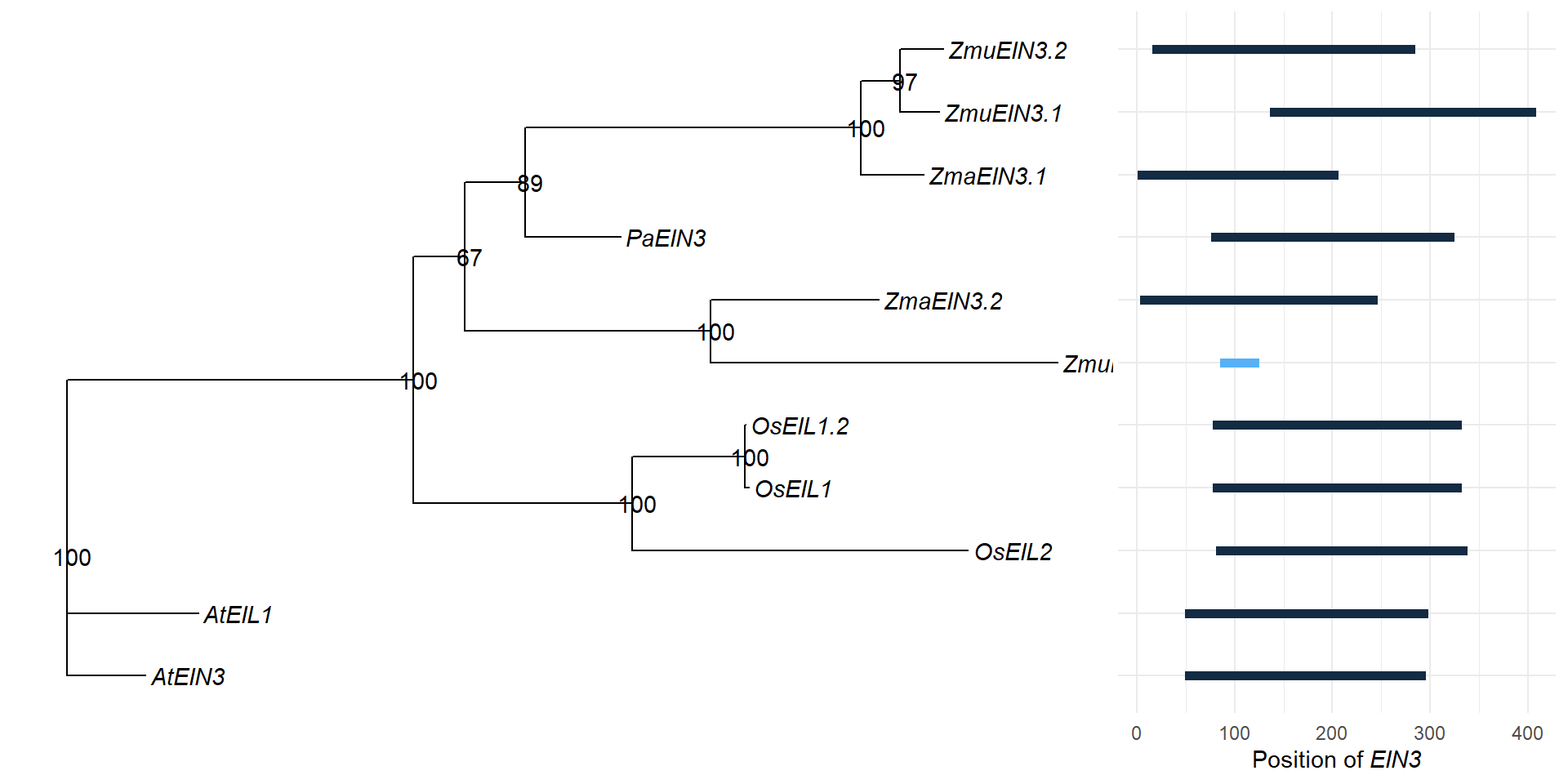
library(patchwork)Warning: package 'patchwork' was built under R version 4.1.1# let's make a patchwork
# PROBLEM: patchwork does not automatically sort, so we'll have to sort the plot `g` manually
plot_order <- p3[['data']] %>% filter(isTip == TRUE) %>% select(label, y) %>% arrange(desc(y))
g <- domains %>% left_join(rename_df, by=c('Gene'='new')) %>% ggplot(aes(y = factor(Gene, levels = plot_order$label), yend=Gene, x=Start, xend=End, color=Evalue)) + geom_segment(size=2) + theme_minimal() + xlab(expression(paste("Position of ", italic("EIN3"))))+ theme(axis.title.y=element_blank(),
axis.text.y = element_blank(),
legend.position='none')
g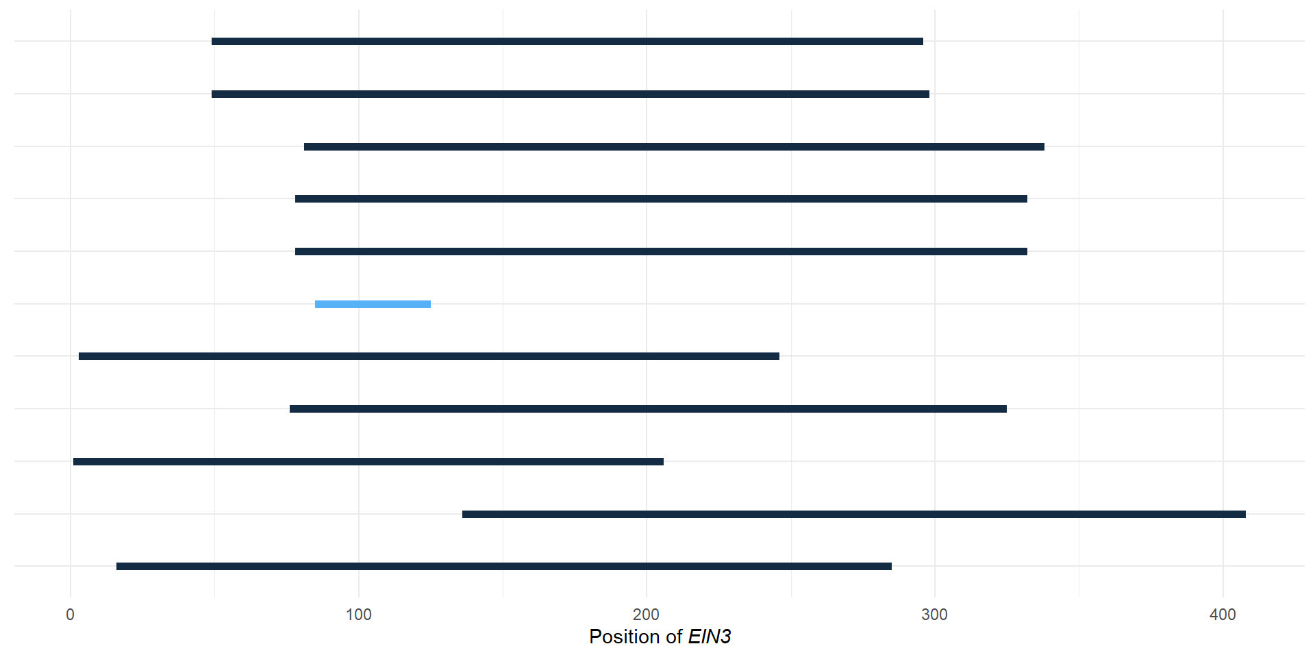
msaplot(p3, './data/EIN3_OG0000629/OG0000629.RiceAraSeagrasses.aln.NamesFixed.fa',
offset = 0.5) + theme(legend.position='none') + g +
plot_layout(widths = c(3.5, 1)) 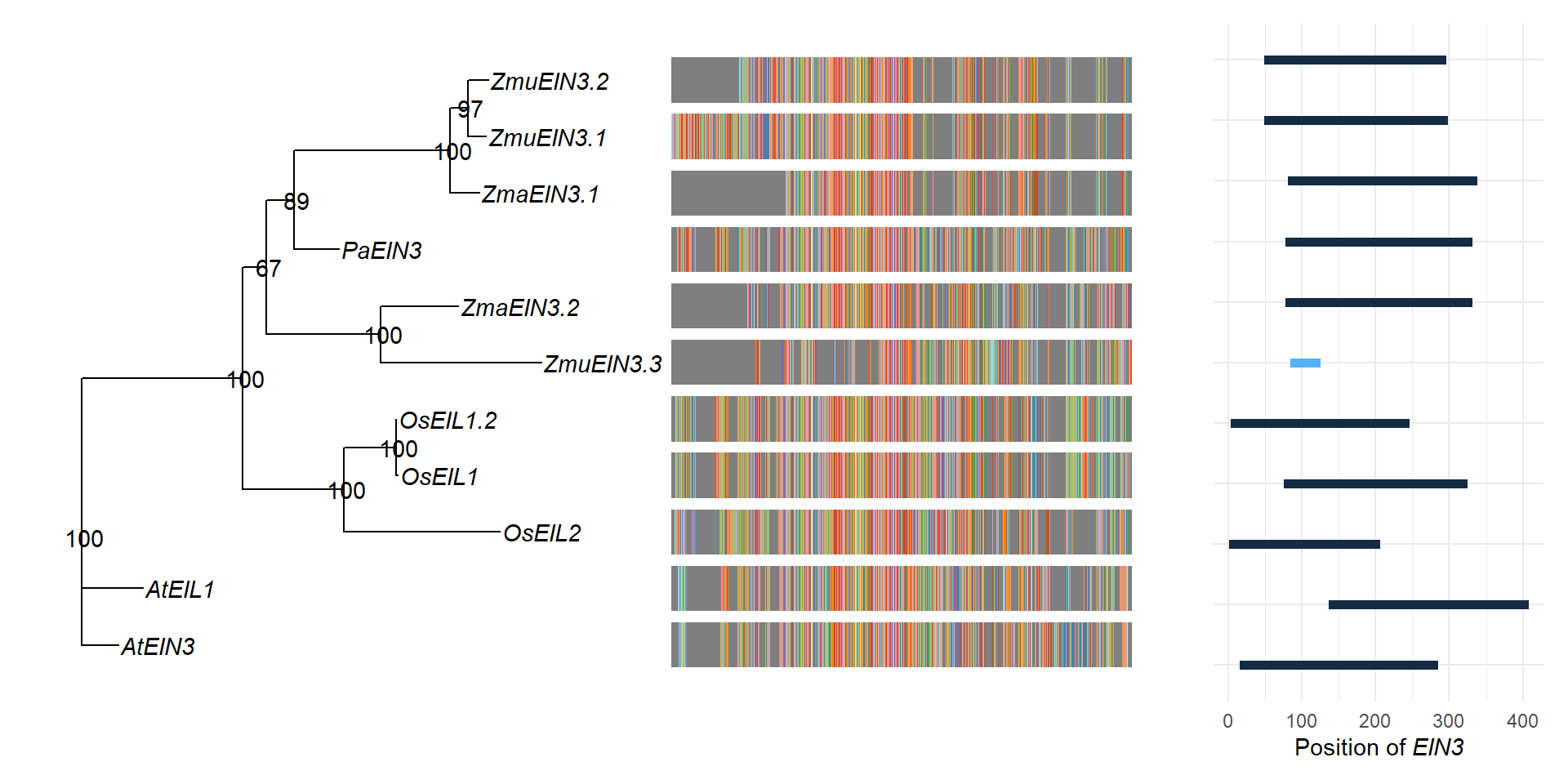
sessionInfo()R version 4.1.0 (2021-05-18)
Platform: x86_64-w64-mingw32/x64 (64-bit)
Running under: Windows 10 x64 (build 19042)
Matrix products: default
locale:
[1] LC_COLLATE=English_Australia.1252 LC_CTYPE=English_Australia.1252
[3] LC_MONETARY=English_Australia.1252 LC_NUMERIC=C
[5] LC_TIME=English_Australia.1252
attached base packages:
[1] stats4 parallel stats graphics grDevices utils datasets
[8] methods base
other attached packages:
[1] patchwork_1.1.1 aplot_0.1.2 treeio_1.16.2
[4] ggtree_3.0.4 ape_5.5 Biostrings_2.60.2
[7] GenomeInfoDb_1.28.4 XVector_0.32.0 IRanges_2.26.0
[10] S4Vectors_0.30.2 BiocGenerics_0.38.0 ggmsa_1.1.5
[13] forcats_0.5.1 stringr_1.4.0 dplyr_1.0.7
[16] purrr_0.3.4 readr_2.1.2 tidyr_1.1.4
[19] tibble_3.1.5 ggplot2_3.3.5 tidyverse_1.3.1
[22] workflowr_1.6.2
loaded via a namespace (and not attached):
[1] colorspace_2.0-2 ellipsis_0.3.2 rprojroot_2.0.2
[4] fs_1.5.0 rstudioapi_0.13 farver_2.1.0
[7] fansi_0.5.0 lubridate_1.8.0 xml2_1.3.2
[10] extrafont_0.17 knitr_1.36 polyclip_1.10-0
[13] jsonlite_1.7.2 broom_0.7.9 Rttf2pt1_1.3.8
[16] dbplyr_2.1.1 ggforce_0.3.3 compiler_4.1.0
[19] httr_1.4.2 backports_1.2.1 assertthat_0.2.1
[22] fastmap_1.1.0 lazyeval_0.2.2 cli_3.2.0
[25] later_1.3.0 tweenr_1.0.2 htmltools_0.5.2
[28] tools_4.1.0 gtable_0.3.0 glue_1.6.2
[31] GenomeInfoDbData_1.2.6 maps_3.4.0 Rcpp_1.0.7
[34] cellranger_1.1.0 jquerylib_0.1.4 vctrs_0.3.8
[37] ggalt_0.4.0 nlme_3.1-152 extrafontdb_1.0
[40] xfun_0.27 rvest_1.0.2 lifecycle_1.0.1
[43] zlibbioc_1.38.0 MASS_7.3-54 scales_1.1.1
[46] hms_1.1.1 promises_1.2.0.1 proj4_1.0-11
[49] RColorBrewer_1.1-2 yaml_2.2.1 R4RNA_1.22.0
[52] ggfun_0.0.5 seqmagick_0.1.5 yulab.utils_0.0.4
[55] sass_0.4.0 stringi_1.7.5 highr_0.9
[58] tidytree_0.3.7 rlang_0.4.12 pkgconfig_2.0.3
[61] bitops_1.0-7 evaluate_0.14 lattice_0.20-44
[64] labeling_0.4.2 cowplot_1.1.1 tidyselect_1.1.1
[67] magrittr_2.0.1 R6_2.5.1 generics_0.1.1
[70] DBI_1.1.1 pillar_1.6.4 haven_2.4.3
[73] whisker_0.4 withr_2.5.0 RCurl_1.98-1.5
[76] ash_1.0-15 modelr_0.1.8 crayon_1.4.1
[79] KernSmooth_2.23-20 utf8_1.2.2 tzdb_0.1.2
[82] rmarkdown_2.11 grid_4.1.0 readxl_1.3.1
[85] git2r_0.28.0 reprex_2.0.1 digest_0.6.28
[88] httpuv_1.6.3 gridGraphics_0.5-1 munsell_0.5.0
[91] ggplotify_0.1.0 bslib_0.3.1