Last updated: 2022-03-30

Checks: 7 0

Knit directory: R_gene_analysis/

This reproducible R Markdown analysis was created with workflowr (version 1.6.2). The Checks tab describes the reproducibility checks that were applied when the results were created. The Past versions tab lists the development history.

R Markdown file: up-to-date

Great! Since the R Markdown file has been committed to the Git repository, you know the exact version of the code that produced these results.

Environment: empty

Great job! The global environment was empty. Objects defined in the global environment can affect the analysis in your R Markdown file in unknown ways. For reproduciblity it’s best to always run the code in an empty environment.

Seed: set.seed(20200917)

The command set.seed(20200917) was run prior to running the code in the R Markdown file. Setting a seed ensures that any results that rely on randomness, e.g. subsampling or permutations, are reproducible.

Session information: recorded

Great job! Recording the operating system, R version, and package versions is critical for reproducibility.

Cache: none

Nice! There were no cached chunks for this analysis, so you can be confident that you successfully produced the results during this run.

File paths: relative

Great job! Using relative paths to the files within your workflowr project makes it easier to run your code on other machines.

Repository version: e025416

Great! You are using Git for version control. Tracking code development and connecting the code version to the results is critical for reproducibility.

The results in this page were generated with repository version e025416. See the Past versions tab to see a history of the changes made to the R Markdown and HTML files.

Note that you need to be careful to ensure that all relevant files for the analysis have been committed to Git prior to generating the results (you can use wflow_publish or wflow_git_commit). workflowr only checks the R Markdown file, but you know if there are other scripts or data files that it depends on. Below is the status of the Git repository when the results were generated:


Ignored files:
    Ignored:    .Rhistory
    Ignored:    .Rproj.user/

Untracked files:
    Untracked:  FigS5.png
    Untracked:  data/Brec_R1.txt
    Untracked:  data/Brec_R2.txt
    Untracked:  data/CR15_R1.txt
    Untracked:  data/CR15_R2.txt
    Untracked:  data/CR_14_R1.txt
    Untracked:  data/CR_14_R2.txt
    Untracked:  data/KS_R1.txt
    Untracked:  data/KS_R2.txt
    Untracked:  data/NBS_PAV.txt.gz
    Untracked:  data/NLR_PAV_GD.txt
    Untracked:  data/NLR_PAV_GM.txt
    Untracked:  data/PAVs_newick.txt
    Untracked:  data/PPR1.txt
    Untracked:  data/PPR2.txt
    Untracked:  data/SNPs_lee.id.biallic_maf_0.05_geno_0.1.vcf.gz
    Untracked:  data/SNPs_newick.txt
    Untracked:  data/bac.txt
    Untracked:  data/brown.txt
    Untracked:  data/cy3.txt
    Untracked:  data/cy5.txt
    Untracked:  data/early.txt
    Untracked:  data/flowerings.txt
    Untracked:  data/foregeye.txt
    Untracked:  data/height.txt
    Untracked:  data/inds.txt
    Untracked:  data/late.txt
    Untracked:  data/mature.txt
    Untracked:  data/motting.txt
    Untracked:  data/mvp.kin.bin
    Untracked:  data/mvp.kin.desc
    Untracked:  data/oil.txt
    Untracked:  data/paperinds.txt
    Untracked:  data/pdh.txt
    Untracked:  data/protein.txt
    Untracked:  data/rust_tan.txt
    Untracked:  data/salt.txt
    Untracked:  data/seedq.txt
    Untracked:  data/seedweight.txt
    Untracked:  data/snp.gds
    Untracked:  data/stem_termination.txt
    Untracked:  data/sudden.txt
    Untracked:  data/virus.txt
    Untracked:  output/FigS5.png
    Untracked:  output/NLR_boxplot_saved.Rds
    Untracked:  output/merged_fig1.png

Unstaged changes:
    Modified:   analysis/total_numbers.Rmd

Note that any generated files, e.g. HTML, png, CSS, etc., are not included in this status report because it is ok for generated content to have uncommitted changes.

These are the previous versions of the repository in which changes were made to the R Markdown (analysis/yield_lm_link.Rmd) and HTML (docs/yield_lm_link.html) files. If you’ve configured a remote Git repository (see ?wflow_git_remote), click on the hyperlinks in the table below to view the files as they were in that past version.

File	Version	Author	Date	Message
Rmd	e025416	Philipp Bayer	2022-03-30	New Fig 1
Rmd	a88c30d	Philipp Bayer	2022-03-01	Add citation
html	548feab	Philipp Bayer	2021-10-18	Build site.
Rmd	7d6bd00	Philipp Bayer	2021-10-18	Minor x-axis inversion
html	5fd2c41	Philipp Bayer	2021-08-10	Build site.
Rmd	265efc1	Philipp Bayer	2021-08-10	Add a new figure
html	901040c	Philipp Bayer	2021-08-10	Build site.
Rmd	bda432c	Philipp Bayer	2021-08-10	Add a new figure
Rmd	b523554	Philipp Bayer	2021-06-12	Add more models
html	b523554	Philipp Bayer	2021-06-12	Add more models
html	af259d3	Philipp Bayer	2021-03-25	Build site.
Rmd	4a9d2c2	Philipp Bayer	2021-03-25	wflow_publish(files = c(“analysis/yield_lm_link.Rmd”))
Rmd	1328f21	Philipp Bayer	2021-03-24	Changed Rmd
html	1c1dab8	Philipp Bayer	2021-03-24	Build site.
Rmd	b1e62b5	Philipp Bayer	2021-03-24	wflow_publish(files = c(“analysis/yield_lm_link.Rmd”))
html	e4a52a8	Philipp Bayer	2021-03-24	Build site.
Rmd	bf0623f	Philipp Bayer	2021-03-24	wflow_publish(files = c(“analysis/yield_lm_link.Rmd”))
Rmd	be81f1b	Philipp Bayer	2021-03-24	missing Modifieds
html	be81f1b	Philipp Bayer	2021-03-24	missing Modifieds
html	0961366	Philipp Bayer	2021-03-24	Build site.
Rmd	e747dc6	Philipp Bayer	2021-03-24	wflow_publish(files = c(“analysis/index.Rmd”, “analysis/yield_lm_link.Rmd”,

knitr::opts_chunk$set(message = FALSE) 

library(tidyverse)

Warning: package 'tidyverse' was built under R version 4.1.2

-- Attaching packages --------------------------------------- tidyverse 1.3.1 --

v ggplot2 3.3.5     v purrr   0.3.4
v tibble  3.1.5     v dplyr   1.0.7
v tidyr   1.1.4     v stringr 1.4.0
v readr   2.1.2     v forcats 0.5.1

Warning: package 'ggplot2' was built under R version 4.1.1

Warning: package 'tibble' was built under R version 4.1.1

Warning: package 'tidyr' was built under R version 4.1.1

Warning: package 'readr' was built under R version 4.1.2

Warning: package 'purrr' was built under R version 4.1.1

Warning: package 'dplyr' was built under R version 4.1.1

Warning: package 'stringr' was built under R version 4.1.1

Warning: package 'forcats' was built under R version 4.1.1

-- Conflicts ------------------------------------------ tidyverse_conflicts() --
x dplyr::filter() masks stats::filter()
x dplyr::lag()    masks stats::lag()

library(patchwork)

Warning: package 'patchwork' was built under R version 4.1.1

library(modelr)

Warning: package 'modelr' was built under R version 4.1.1

library(sjPlot)

Warning: package 'sjPlot' was built under R version 4.1.2

Learn more about sjPlot with 'browseVignettes("sjPlot")'.

library(ggsci)

Warning: package 'ggsci' was built under R version 4.1.2

library(dabestr)

Warning: package 'dabestr' was built under R version 4.1.2

Loading required package: magrittr

Warning: package 'magrittr' was built under R version 4.1.1


Attaching package: 'magrittr'

The following object is masked from 'package:purrr':

    set_names

The following object is masked from 'package:tidyr':

    extract

library(cowplot)

Warning: package 'cowplot' was built under R version 4.1.1


Attaching package: 'cowplot'

The following objects are masked from 'package:sjPlot':

    plot_grid, save_plot

The following object is masked from 'package:patchwork':

    align_plots

library(ggsignif)

Warning: package 'ggsignif' was built under R version 4.1.2

library(ggforce)

Warning: package 'ggforce' was built under R version 4.1.2

library(lme4)

Warning: package 'lme4' was built under R version 4.1.2

Loading required package: Matrix


Attaching package: 'Matrix'

The following objects are masked from 'package:tidyr':

    expand, pack, unpack

library(lmerTest)

Warning: package 'lmerTest' was built under R version 4.1.2


Attaching package: 'lmerTest'

The following object is masked from 'package:lme4':

    lmer

The following object is masked from 'package:stats':

    step

library(dotwhisker)

Warning: package 'dotwhisker' was built under R version 4.1.2

library(pals)

Warning: package 'pals' was built under R version 4.1.2

theme_set(theme_cowplot())
library(RColorBrewer)

Warning: package 'RColorBrewer' was built under R version 4.1.1

library(countrycode)

Warning: package 'countrycode' was built under R version 4.1.2

library(broom)

Warning: package 'broom' was built under R version 4.1.1


Attaching package: 'broom'

The following object is masked from 'package:modelr':

    bootstrap

Data loading

npg_col = pal_npg("nrc")(9)
col_list <- c(`Wild`=npg_col[8],
   Landrace = npg_col[3],
  `Old cultivar`=npg_col[2],
  `Modern cultivar`=npg_col[4])

pav_table <- read_tsv('./data/soybean_pan_pav.matrix_gene.txt.gz')

nbs <- read_tsv('./data/Lee.NBS.candidates.lst', col_names = c('Name', 'Class'))
nbs

# A tibble: 486 x 2
   Name                   Class
   <chr>                  <chr>
 1 UWASoyPan00953.t1      CN   
 2 GlymaLee.13G222900.1.p CN   
 3 GlymaLee.18G227000.1.p CN   
 4 GlymaLee.18G080600.1.p CN   
 5 GlymaLee.20G036200.1.p CN   
 6 UWASoyPan01876.t1      CN   
 7 UWASoyPan04211.t1      CN   
 8 GlymaLee.19G105400.1.p CN   
 9 GlymaLee.18G085100.1.p CN   
10 GlymaLee.11G142600.1.p CN   
# ... with 476 more rows

# have to remove the .t1s 
nbs$Name <- gsub('.t1','', nbs$Name)
nbs_pav_table <- pav_table %>% filter(Individual %in% nbs$Name)

names <- c()
presences <- c()

for (i in seq_along(nbs_pav_table)){
  if ( i == 1) next
  thisind <- colnames(nbs_pav_table)[i]
  pavs <- nbs_pav_table[[i]]
  presents <- sum(pavs)
  names <- c(names, thisind)
  presences <- c(presences, presents)
}
nbs_res_tibb <- new_tibble(list(names = names, presences = presences))

# let's make the same table for all genes too
names <- c()
presences <- c()

for (i in seq_along(pav_table)){
  if ( i == 1) next
  thisind <- colnames(pav_table)[i]
  pavs <- pav_table[[i]]
  presents <- sum(pavs)
  names <- c(names, thisind)
  presences <- c(presences, presents)
}
res_tibb <- new_tibble(list(names = names, presences = presences))

groups <- read_csv('./data/Table_of_cultivar_groups.csv')
groups <- groups %>% dplyr::rename(Group = `Group in violin table`)
groups <- groups %>% 
  mutate(Group = str_replace_all(Group, 'landrace', 'Landrace')) %>%
  mutate(Group = str_replace_all(Group, 'Old_cultivar', 'Old cultivar')) %>%
  mutate(Group = str_replace_all(Group, 'Modern_cultivar', 'Modern cultivar')) %>%
  mutate(Group = str_replace_all(Group, 'Wild-type', 'Wild'))

groups$Group <-
  factor(
    groups$Group,
    levels = c('Wild',
               'Landrace',
               'Old cultivar',
               'Modern cultivar')
  )

nbs_joined_groups <-
  inner_join(nbs_res_tibb, groups, by = c('names' = 'Data-storage-ID'))
all_joined_groups <-
    inner_join(res_tibb, groups, by = c('names' = 'Data-storage-ID'))

country <- read_csv('./data/Cultivar_vs_country.csv')


names(country) <- c('names', 'PI-ID', 'Country')

# fix weird ND issue
country <- country %>% mutate(Country = na_if(Country, 'ND')) %>% 
  mutate(Country = str_replace_all(Country, 'Costa', 'Costa Rica'))

Linking with yield

Can we link the trajectory of NLR genes with the trajectory of yield across the history of soybean breeding? let’s make a simple regression for now

Yield

yield <- read_tsv('./data/yield.txt')
yield_join <- inner_join(nbs_res_tibb, yield, by=c('names'='Line'))

Protein

protein <- read_tsv('./data/protein_phenotype.txt')
protein_join <- left_join(nbs_res_tibb, protein, by=c('names'='Line')) %>% filter(!is.na(Protein))

Seed weight

Let’s look at seed weight:

seed_weight <- read_tsv('./data/Seed_weight_Phenotype.txt', col_names = c('names', 'wt'))
seed_join <- left_join(nbs_res_tibb, seed_weight) %>% filter(!is.na(wt))

Oil content

And now let’s look at the oil phenotype:

oil <- read_tsv('./data/oil_phenotype.txt')
oil_join <- left_join(nbs_res_tibb, oil, by=c('names'='Line')) %>% filter(!is.na(Oil))
oil_join

# A tibble: 962 x 3
   names presences   Oil
   <chr>     <dbl> <dbl>
 1 AB-01       445  17.6
 2 AB-02       454  16.8
 3 BR-24       455  20.6
 4 ESS         454  20.9
 5 For         448  21  
 6 HN001       448  23.6
 7 HN002       444  18.5
 8 HN003       446  17.5
 9 HN004       442  18.9
10 HN005       440  15.5
# ... with 952 more rows

Basic lm()

These results form the basis of the paper.

Yield

yield_nbs_joined_groups <- nbs_joined_groups %>% inner_join(yield_join, by = 'names') 
yield_nbs_joined_groups$Yield2 <-scale(yield_nbs_joined_groups$Yield, center=T, scale=T)

yield_all_joined_groups <- all_joined_groups %>% inner_join(yield_join, by = 'names')

yield_country_nbs_joined_groups <- yield_nbs_joined_groups %>% inner_join(country)
yield_country_all_joined_groups <- yield_all_joined_groups %>% inner_join(country)
yield_country_nbs_joined_groups$Count <- yield_country_nbs_joined_groups$presences.y
yield_country_all_joined_groups$Count <- yield_country_all_joined_groups$presences.y

yield_country_all_joined_groups %>% dplyr::count(Country)

# A tibble: 40 x 2
   Country        n
   <chr>      <int>
 1 Algeria        3
 2 Argentina      2
 3 Australia      1
 4 Austria        1
 5 Belgium        2
 6 Brazil         1
 7 Bulgaria       1
 8 Canada         5
 9 China        410
10 Costa Rica     1
# ... with 30 more rows

lm_model <- lm(Yield ~ Count +  Group, data = yield_country_nbs_joined_groups) 
summary(lm_model)


Call:
lm(formula = Yield ~ Count + Group, data = yield_country_nbs_joined_groups)

Residuals:
     Min       1Q   Median       3Q      Max 
-2.47398 -0.52358  0.02648  0.53660  2.14648 

Coefficients:
                      Estimate Std. Error t value Pr(>|t|)    
(Intercept)          10.985573   2.532389   4.338 1.64e-05 ***
Count                -0.019960   0.005694  -3.505 0.000483 ***
GroupOld cultivar    -0.198279   0.137005  -1.447 0.148255    
GroupModern cultivar  1.080136   0.111621   9.677  < 2e-16 ***
---
Signif. codes:  0 '***' 0.001 '**' 0.01 '*' 0.05 '.' 0.1 ' ' 1

Residual standard error: 0.768 on 737 degrees of freedom
Multiple R-squared:  0.1412,    Adjusted R-squared:  0.1377 
F-statistic: 40.41 on 3 and 737 DF,  p-value: < 2.2e-16

clm_model <- lm(Yield ~ Count +  Group + Country, data = yield_country_nbs_joined_groups) 
summary(clm_model)


Call:
lm(formula = Yield ~ Count + Group + Country, data = yield_country_nbs_joined_groups)

Residuals:
     Min       1Q   Median       3Q      Max 
-2.25859 -0.39669  0.00554  0.45439  2.09622 

Coefficients:
                      Estimate Std. Error t value Pr(>|t|)    
(Intercept)           9.306701   2.552306   3.646 0.000286 ***
Count                -0.016068   0.005701  -2.818 0.004965 ** 
GroupOld cultivar    -0.217698   0.139274  -1.563 0.118490    
GroupModern cultivar  0.801209   0.214539   3.735 0.000204 ***
CountryArgentina     -0.599057   0.693473  -0.864 0.387970    
CountryAustralia     -0.684304   0.834828  -0.820 0.412674    
CountryAustria        0.415356   0.834277   0.498 0.618739    
CountryBelgium       -0.290712   0.659563  -0.441 0.659522    
CountryBrazil        -0.734304   0.834828  -0.880 0.379390    
CountryBulgaria      -0.418916   0.834536  -0.502 0.615846    
CountryCanada        -0.151286   0.557169  -0.272 0.786068    
CountryChina         -0.028384   0.418992  -0.068 0.946009    
CountryCosta Rica     0.781084   0.834536   0.936 0.349627    
CountryFormer Serbia  1.044147   0.861446   1.212 0.225895    
CountryFrance         0.309458   0.551920   0.561 0.575188    
CountryGeorgia        0.814118   0.659799   1.234 0.217665    
CountryGermany       -0.241499   0.556404  -0.434 0.664398    
CountryHungary        0.613026   0.552057   1.110 0.267197    
CountryIndia         -1.154389   0.552312  -2.090 0.036974 *  
CountryIndonesia     -1.244474   0.552057  -2.254 0.024494 *  
CountryItaly          0.479122   0.845855   0.566 0.571282    
CountryJapan         -0.335560   0.427004  -0.786 0.432227    
CountryKorea         -0.230379   0.426146  -0.541 0.588951    
CountryKyrgyzstan     0.705356   0.834277   0.845 0.398142    
CountryMoldova        0.021216   0.498774   0.043 0.966083    
CountryMorocco        0.830308   0.838267   0.991 0.322275    
CountryMyanmar       -1.112120   0.660646  -1.683 0.092754 .  
CountryNepal         -0.445542   0.659635  -0.675 0.499624    
CountryNetherlands   -0.710712   0.834283  -0.852 0.394575    
CountryPakistan      -2.183188   0.835419  -2.613 0.009163 ** 
CountryPeru          -1.182508   0.834381  -1.417 0.156868    
CountryPoland         0.955696   0.834828   1.145 0.252697    
CountryRomania        1.153091   0.510943   2.257 0.024334 *  
CountryRussia         0.539649   0.432796   1.247 0.212862    
CountrySerbia         0.221424   0.659596   0.336 0.737202    
CountrySouth Africa  -0.600125   0.861382  -0.697 0.486225    
CountrySweden        -0.766382   0.592628  -1.293 0.196378    
CountryTaiwan        -0.656968   0.528544  -1.243 0.214299    
CountryUkraine        0.723560   0.834491   0.867 0.386207    
CountryUSA            0.345864   0.463385   0.746 0.455689    
CountryUzbekistan     0.315016   0.834699   0.377 0.705992    
CountryVietnam       -0.693042   0.551920  -1.256 0.209653    
---
Signif. codes:  0 '***' 0.001 '**' 0.01 '*' 0.05 '.' 0.1 ' ' 1

Residual standard error: 0.7225 on 689 degrees of freedom
  (10 observations deleted due to missingness)
Multiple R-squared:  0.2829,    Adjusted R-squared:  0.2403 
F-statistic: 6.631 on 41 and 689 DF,  p-value: < 2.2e-16

yieldmod <- clm_model

interlm_model <- lm(Yield ~ Count * Group, data = yield_country_nbs_joined_groups) 
summary(interlm_model)


Call:
lm(formula = Yield ~ Count * Group, data = yield_country_nbs_joined_groups)

Residuals:
     Min       1Q   Median       3Q      Max 
-2.38311 -0.51569  0.01947  0.53258  2.13947 

Coefficients:
                           Estimate Std. Error t value Pr(>|t|)    
(Intercept)                 9.62255    2.70414   3.558 0.000397 ***
Count                      -0.01690    0.00608  -2.779 0.005598 ** 
GroupOld cultivar          18.63259   11.02113   1.691 0.091333 .  
GroupModern cultivar        5.56130   10.01054   0.556 0.578692    
Count:GroupOld cultivar    -0.04234    0.02478  -1.709 0.087920 .  
Count:GroupModern cultivar -0.01012    0.02263  -0.447 0.654959    
---
Signif. codes:  0 '***' 0.001 '**' 0.01 '*' 0.05 '.' 0.1 ' ' 1

Residual standard error: 0.7674 on 735 degrees of freedom
Multiple R-squared:  0.1448,    Adjusted R-squared:  0.139 
F-statistic: 24.88 on 5 and 735 DF,  p-value: < 2.2e-16

tab_model(clm_model, p.val='kr', digits=3)

Warning: 'ci_method' must be one of 'residual', 'wald', normal', 'profile', 'boot',
  'uniroot', 'betwithin' or 'ml1'. Using 'wald' now.

	Yield
Predictors	Estimates	CI	p
(Intercept)	9.307	4.295 – 14.318	<0.001
Count	-0.016	-0.027 – -0.005	0.005
Group [Old cultivar]	-0.218	-0.491 – 0.056	0.118
Group [Modern cultivar]	0.801	0.380 – 1.222	<0.001
Country [Argentina]	-0.599	-1.961 – 0.763	0.388
Country [Australia]	-0.684	-2.323 – 0.955	0.413
Country [Austria]	0.415	-1.223 – 2.053	0.619
Country [Belgium]	-0.291	-1.586 – 1.004	0.660
Country [Brazil]	-0.734	-2.373 – 0.905	0.379
Country [Bulgaria]	-0.419	-2.057 – 1.220	0.616
Country [Canada]	-0.151	-1.245 – 0.943	0.786
Country [China]	-0.028	-0.851 – 0.794	0.946
Country [Costa Rica]	0.781	-0.857 – 2.420	0.350
Country [Former Serbia]	1.044	-0.647 – 2.736	0.226
Country [France]	0.309	-0.774 – 1.393	0.575
Country [Georgia]	0.814	-0.481 – 2.110	0.218
Country [Germany]	-0.241	-1.334 – 0.851	0.664
Country [Hungary]	0.613	-0.471 – 1.697	0.267
Country [India]	-1.154	-2.239 – -0.070	0.037
Country [Indonesia]	-1.244	-2.328 – -0.161	0.024
Country [Italy]	0.479	-1.182 – 2.140	0.571
Country [Japan]	-0.336	-1.174 – 0.503	0.432
Country [Korea]	-0.230	-1.067 – 0.606	0.589
Country [Kyrgyzstan]	0.705	-0.933 – 2.343	0.398
Country [Moldova]	0.021	-0.958 – 1.001	0.966
Country [Morocco]	0.830	-0.816 – 2.476	0.322
Country [Myanmar]	-1.112	-2.409 – 0.185	0.093
Country [Nepal]	-0.446	-1.741 – 0.850	0.500
Country [Netherlands]	-0.711	-2.349 – 0.927	0.395
Country [Pakistan]	-2.183	-3.823 – -0.543	0.009
Country [Peru]	-1.183	-2.821 – 0.456	0.157
Country [Poland]	0.956	-0.683 – 2.595	0.253
Country [Romania]	1.153	0.150 – 2.156	0.024
Country [Russia]	0.540	-0.310 – 1.389	0.213
Country [Serbia]	0.221	-1.074 – 1.516	0.737
Country [South Africa]	-0.600	-2.291 – 1.091	0.486
Country [Sweden]	-0.766	-1.930 – 0.397	0.196
Country [Taiwan]	-0.657	-1.695 – 0.381	0.214
Country [Ukraine]	0.724	-0.915 – 2.362	0.386
Country [USA]	0.346	-0.564 – 1.256	0.456
Country [Uzbekistan]	0.315	-1.324 – 1.954	0.706
Country [Vietnam]	-0.693	-1.777 – 0.391	0.210
Observations	731
R² / R² adjusted	0.283 / 0.240

newdat <-cbind(yield_country_all_joined_groups %>% filter(!is.na(Country)), pred = predict(clm_model))

# I want only every second, stronger color of the Paired scheme
mycol <- brewer.pal(n = 12, name = "Paired")[seq(2, 12, 2)]

newdat %>% mutate(
  Country2 = case_when (
  Country == 'USA' ~ 'USA',
  Country == 'China' ~ 'China',
  Country == 'Korea' ~ 'Korea',
  Country == 'Japan' ~ 'Japan',
  Country == 'Russia' ~ 'Russia',
  TRUE ~ 'Rest'
  )
  ) %>%
  mutate(Country2 = factor(
  Country2,
  levels = c('China', 'Japan', 'Korea', 'Russia', 'USA', 'Rest')
  )) %>%
  ggplot(aes(x = Count, y = pred, color = Country2)) +
  facet_wrap(~ Group, nrow = 1) +  
  geom_point(aes(y = Yield, color = Country2),
    alpha = 0.8,
    size = 2) +
  geom_line(aes(y=pred, group=interaction(Group, Country),colour=Country2), size=1.5)+
  theme_minimal_hgrid() +
  xlab('Gene count') +
  ylab(expression(paste('Yield [Mg ', ha ^ -1, ']'))) +
  scale_color_manual(values = mycol) +
  #xlim(c(47.900, 49.700)) +
  labs(color = "Country") +
  theme(panel.spacing = unit(0.9, "lines"),
  axis.text.x = element_text(size = 10))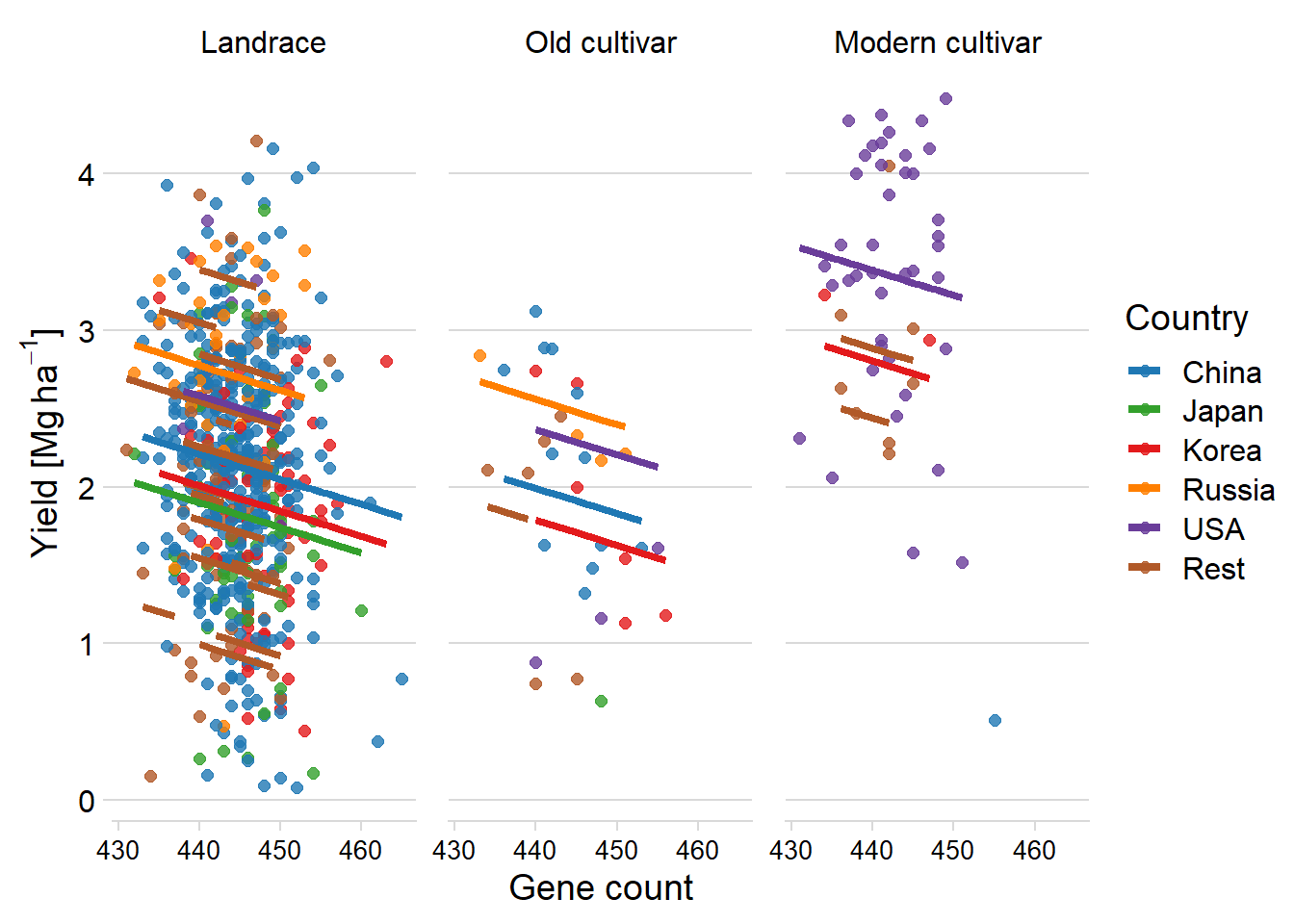

Oh wow, that looks very similar to the lme4 results.

By what percentage does the predicted yield change for each group?

plot_model(clm_model, type = "pred", terms = c("Count", "Group"))$data

# Predicted values of Yield

# Group = Landrace

Count | Predicted | group_col |       95% CI
--------------------------------------------
  430 |      2.37 |  Landrace | [2.19, 2.55]
  436 |      2.27 |  Landrace | [2.15, 2.39]
  442 |      2.18 |  Landrace | [2.10, 2.25]
  448 |      2.08 |  Landrace | [2.00, 2.16]
  454 |      1.98 |  Landrace | [1.86, 2.11]
  466 |      1.79 |  Landrace | [1.54, 2.04]

# Group = Old cultivar

Count | Predicted |    group_col |       95% CI
-----------------------------------------------
  430 |      2.15 | Old cultivar | [1.83, 2.47]
  436 |      2.05 | Old cultivar | [1.77, 2.34]
  442 |      1.96 | Old cultivar | [1.68, 2.23]
  448 |      1.86 | Old cultivar | [1.59, 2.14]
  454 |      1.77 | Old cultivar | [1.47, 2.06]
  466 |      1.57 | Old cultivar | [1.21, 1.94]

# Group = Modern cultivar

Count | Predicted |       group_col |       95% CI
--------------------------------------------------
  430 |      3.17 | Modern cultivar | [2.72, 3.62]
  436 |      3.07 | Modern cultivar | [2.64, 3.50]
  442 |      2.98 | Modern cultivar | [2.55, 3.40]
  448 |      2.88 | Modern cultivar | [2.45, 3.31]
  454 |      2.78 | Modern cultivar | [2.34, 3.23]
  466 |      2.59 | Modern cultivar | [2.09, 3.09]

Adjusted for:
* Country = China

ranges_pret <- list(land = c(1.79, 2.37), old = c(1.57, 2.15), modern = c(2.59, 3.17))
sapply(ranges_pret, diff)

  land    old modern 
  0.58   0.58   0.58

So the effect is around 0.58 per group

fig2 <- plot_model(clm_model, type = "pred", terms = c("Count", "Group"), show.data=F) +
  theme_minimal_hgrid() +
  #scale_fill_manual(values = col_list) +
  #scale_color_manual(values = col_list) +
  xlab('NLR count') + 
  ylab((expression(paste('Yield [Mg ', ha^-1, ']')))) +
  theme(plot.title=element_blank())
fig2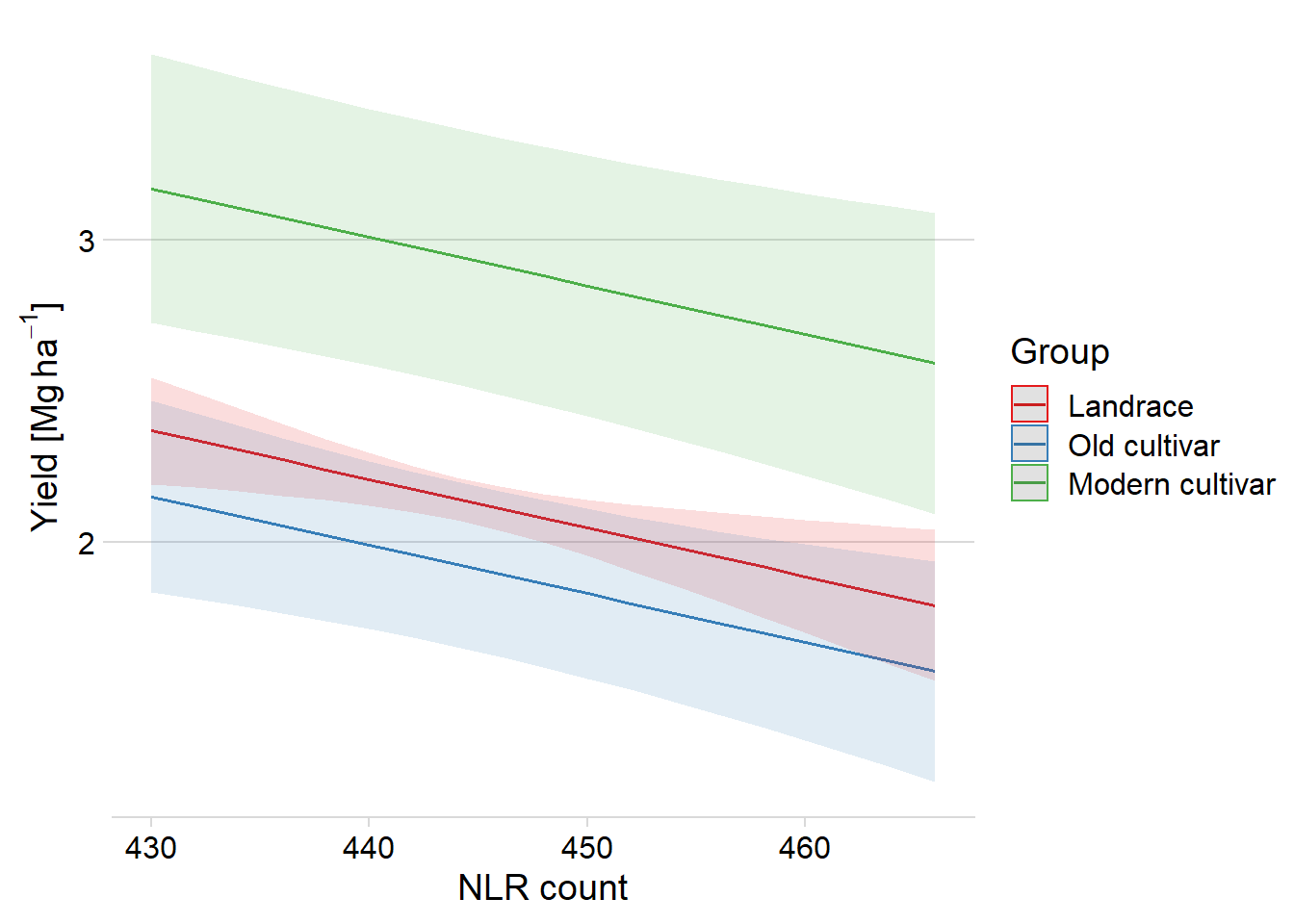

We can revert this plot too:

plot_model(clm_model, type = "pred", terms = c("Count", "Group"), show.data=F) +
  theme_minimal_hgrid() +
  #scale_fill_manual(values = col_list) +
  #scale_color_manual(values = col_list) +
  xlab('NLR count') + 
  ylab((expression(paste('Yield [Mg ', ha^-1, ']')))) +
  theme(plot.title=element_blank()) +
  scale_x_reverse()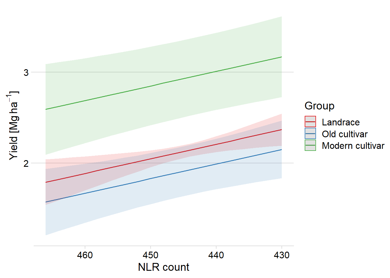

qqnorm(resid(clm_model))
qqline(resid(clm_model))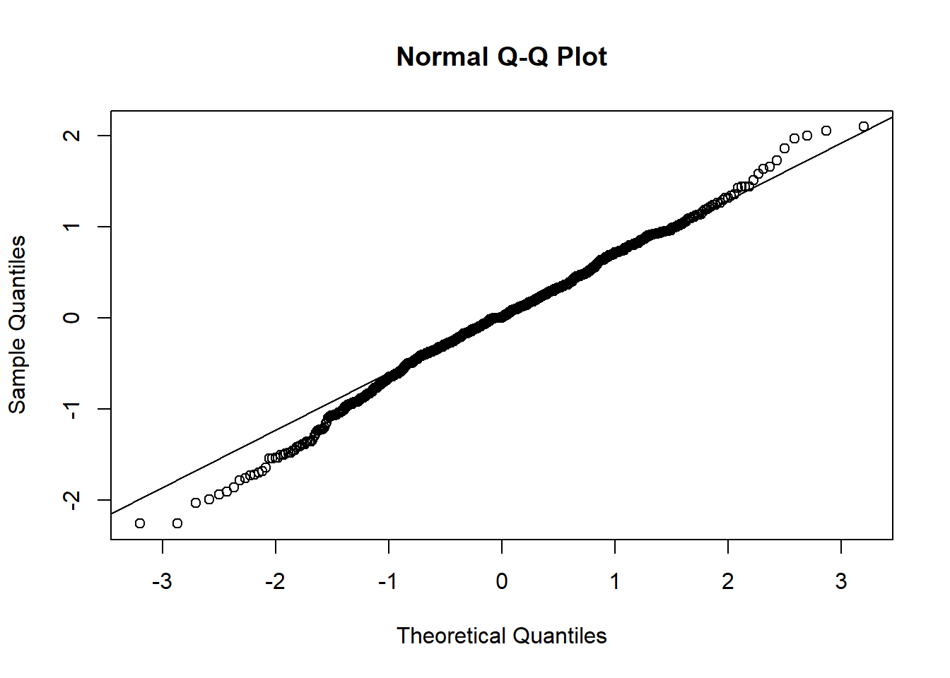

plot(resid(clm_model))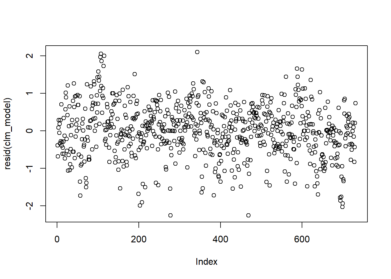

theme_set(theme_sjplot())

fig4 <- plot_model(clm_model, show.values = TRUE, value.offset = .3, terms=c('GroupOld cultivar', 'Count', 'GroupModern cultivar'))
fig4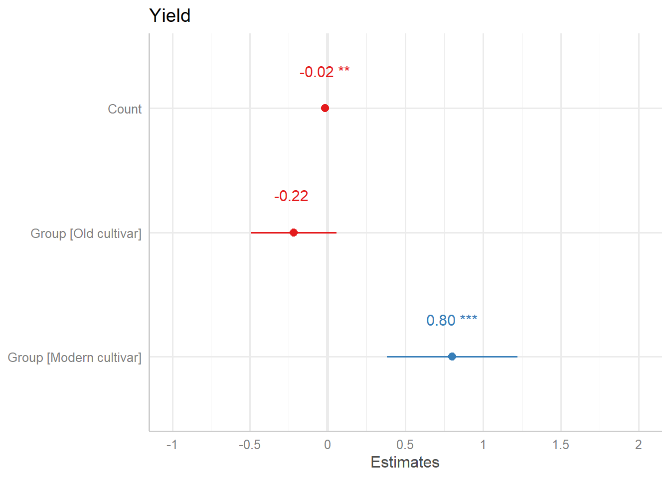

All terms in the model:

plot_model(clm_model, type = "std", show.values = TRUE, value.offset = .3)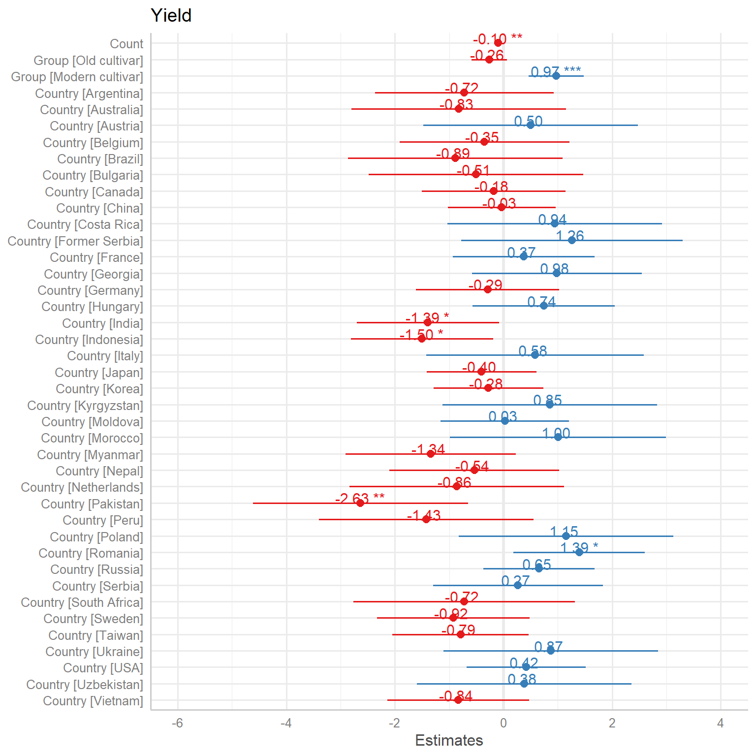

Only groups and count:

plot_model(clm_model, type = "std", show.values = TRUE, value.offset = .3, terms=c('GroupOld cultivar', 'Count', 'GroupModern cultivar'))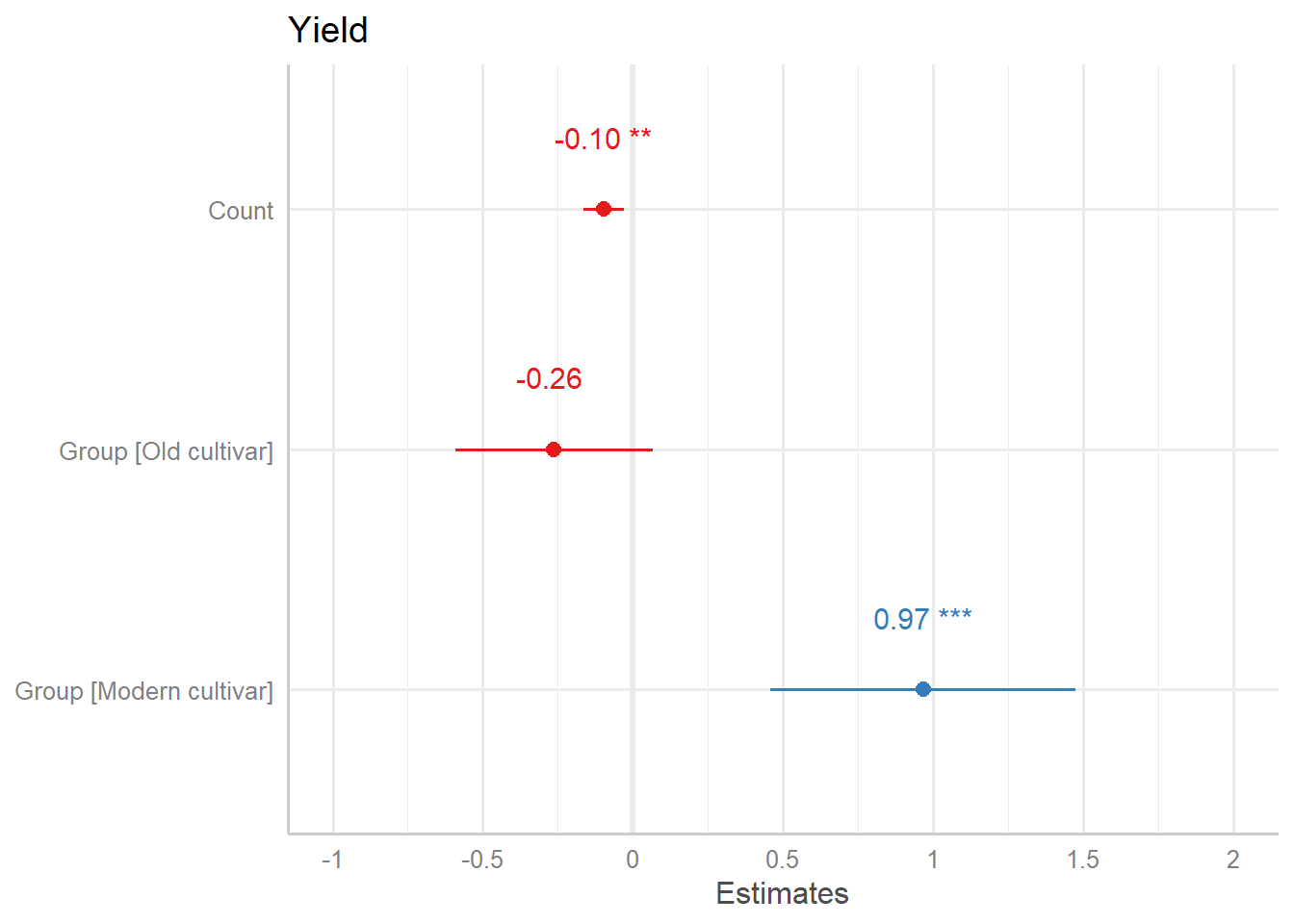

Only countries and count:

theme_set(theme_sjplot())

p <- plot_model(clm_model, type = "std", show.values = TRUE, value.offset = .6, auto.label = F, terms=c(names(clm_model$coefficients)[2], names(clm_model$coefficients)[-1:-4])) +
      scale_x_discrete(expand = expansion(mult=0.05)) +
  theme(axis.text.y = element_text(colour = 'black'))
p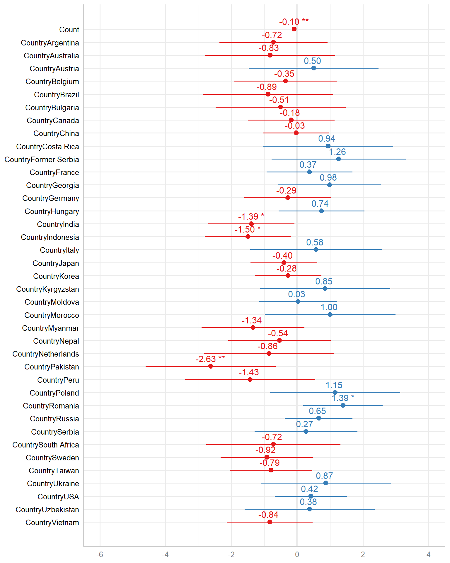

cowplot::save_plot(filename = 'output/FigS5.png', p, base_height = 3.71*2)

Let’s plot while having no colors for the countries:

newdatlm <-cbind(yield_country_nbs_joined_groups, pred = predict(lm_model))

fig1 <- newdatlm %>% mutate(
  Country2 = case_when (
  Country == 'USA' ~ 'USA',
  Country == 'China' ~ 'China',
  Country == 'Korea' ~ 'Korea',
  Country == 'Japan' ~ 'Japan',
  Country == 'Russia' ~ 'Russia',
  TRUE ~ 'Rest'
  )
  ) %>%
  mutate(Country2 = factor(
  Country2,
  levels = c('China', 'Japan', 'Korea', 'Russia', 'USA', 'Rest')
  )) %>%
  ggplot(aes(x = Count, y = pred, color = Country2)) +
  facet_wrap(~ Group, nrow = 1) +  
  geom_point(aes(y = Yield, color = Country2),
    alpha = 0.8,
    size = 2) +
  geom_line(aes(y=pred), color='black', size=1.5)+
  theme_minimal_hgrid() +
  xlab('Gene count') +
  ylab(expression(paste('Yield [Mg ', ha ^ -1, ']'))) +
  scale_color_manual(values = mycol) +
  #xlim(c(47.900, 49.700)) +
  labs(color = "Country") +
  theme(panel.spacing = unit(0.9, "lines"),
  axis.text.x = element_text(size = 10))
fig1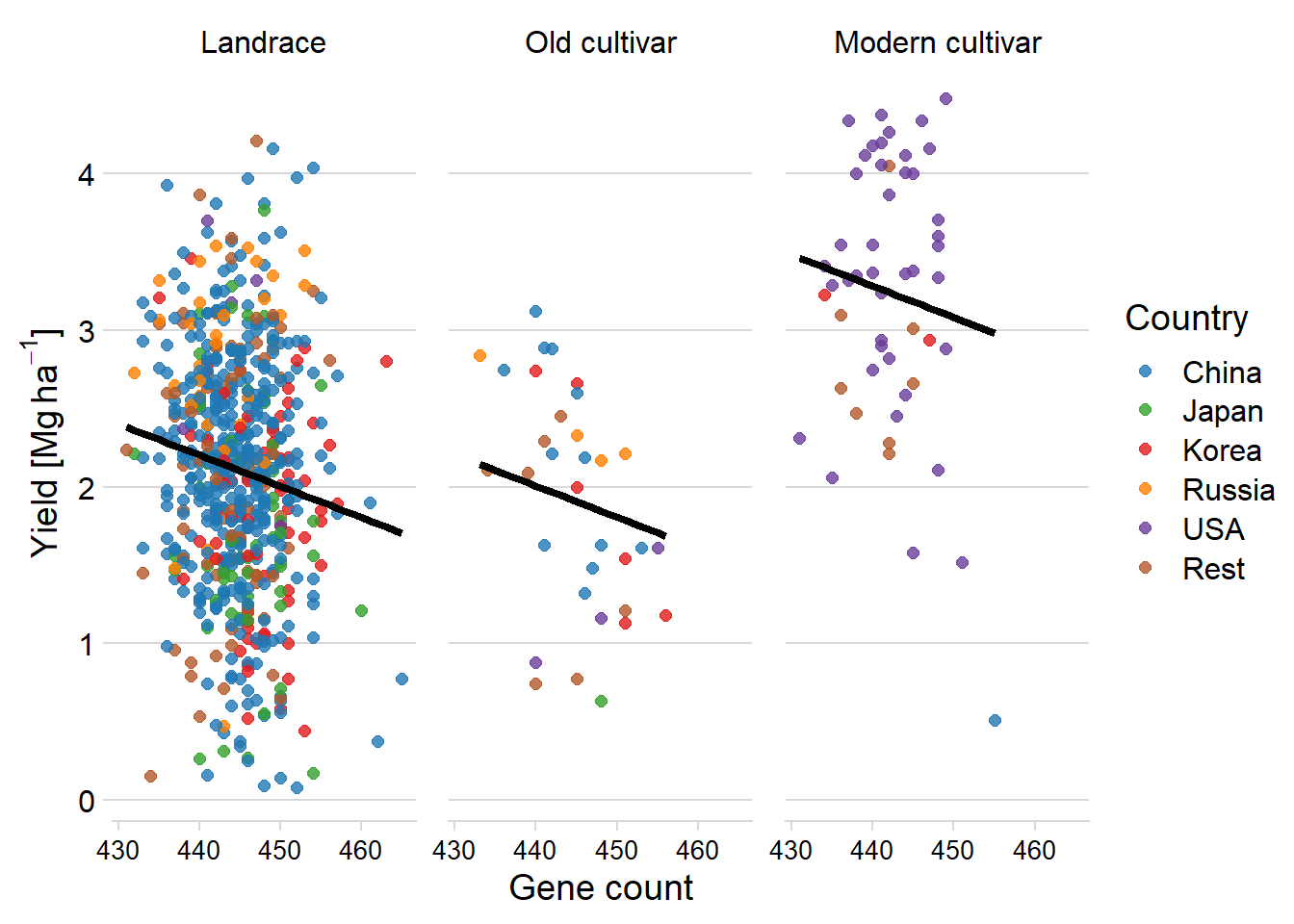

Let’s use this as figure 1.

We can also reverse the x-axis:

newdatlm %>% mutate(
  Country2 = case_when (
  Country == 'USA' ~ 'USA',
  Country == 'China' ~ 'China',
  Country == 'Korea' ~ 'Korea',
  Country == 'Japan' ~ 'Japan',
  Country == 'Russia' ~ 'Russia',
  TRUE ~ 'Rest'
  )
  ) %>%
  mutate(Country2 = factor(
  Country2,
  levels = c('China', 'Japan', 'Korea', 'Russia', 'USA', 'Rest')
  )) %>%
  ggplot(aes(x = Count, y = pred, color = Country2)) +
  facet_wrap(~ Group, nrow = 1) +  
  geom_point(aes(y = Yield, color = Country2),
    alpha = 0.8,
    size = 2) +
  geom_line(aes(y=pred), color='black', size=1.5)+
  theme_minimal_hgrid() +
  xlab('Gene count') +
  ylab(expression(paste('Yield [Mg ', ha ^ -1, ']'))) +
  scale_color_manual(values = mycol) +
  #xlim(c(47.900, 49.700)) +
  labs(color = "Country") +
  theme(panel.spacing = unit(0.9, "lines"),
  axis.text.x = element_text(size = 10)) +
  scale_x_reverse()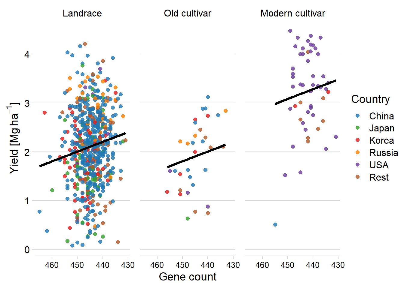

Let’s nest the countries and run one lm each

First, let’s look at the models

 six_country_table <- newdat %>% mutate(
  Country2 = case_when (
  Country == 'USA' ~ 'USA',
  Country == 'China' ~ 'China',
  Country == 'Korea' ~ 'Korea',
  Country == 'Japan' ~ 'Japan',
  Country == 'Russia' ~ 'Russia',
  TRUE ~ 'Rest'
  )
  )
  
models <- six_country_table %>% 
  mutate(Country2 = factor(
  Country2,
  levels = c('China', 'Japan', 'Korea', 'Russia', 'USA', 'Rest')
  )) %>% 
  plyr::dlply(c('Country2'), function(df)  
    lm(Yield ~ Count, data=df)
  )

model_tibble <- tibble(id = names(models), model=models)

plot_models(models, m.labels = names(models), p.shape=TRUE) +
  scale_colour_manual(values = mycol)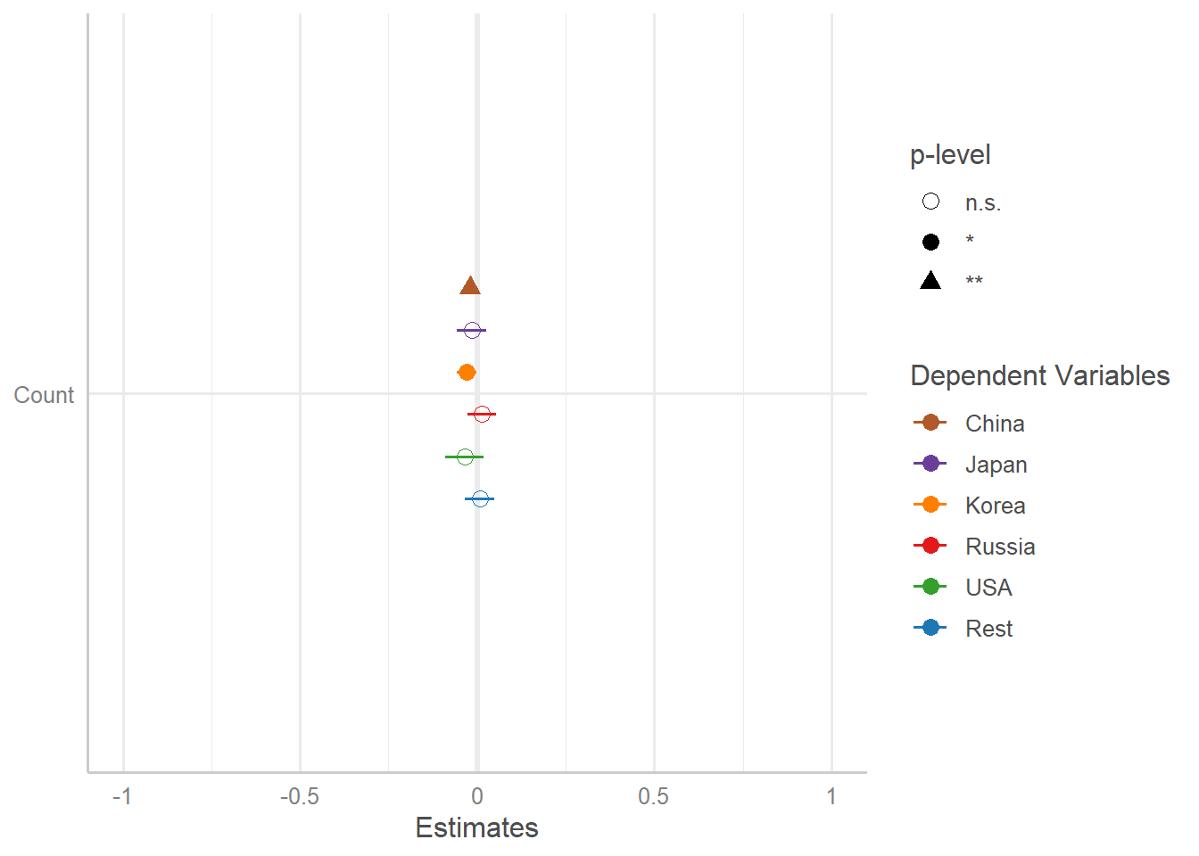

mymodel <-  function(df) { lm(Yield ~ Count, data=df) }

results <- six_country_table %>% nest(data = -c(Group, Country2)) %>% 
  mutate(model = map(data, mymodel)) %>% 
  mutate(pred = map2(data, model, add_predictions))

Warning in predict.lm(model, data): prediction from a rank-deficient fit may be
misleading

Warning in predict.lm(model, data): prediction from a rank-deficient fit may be
misleading

results %>% 
  unnest(pred) %>% 
  select(-c(data, model)) %>% 
  ggplot(aes(x = Count, y = pred, color = Country2)) +
  facet_wrap(~ Group, nrow = 1) +  
  geom_point(aes(y = Yield, color = Country2),
    alpha = 0.8,
    size = 2) +
  geom_line(aes(y=pred, group=interaction(Group, Country),colour=Country2), size=1.5)+
  theme_minimal_hgrid() +
  xlab('Gene count') +
  ylab(expression(paste('Yield [Mg ', ha ^ -1, ']'))) +
  scale_color_manual(values = mycol) +
  #xlim(c(47.900, 49.700)) +
  labs(color = "Country") +
  theme(panel.spacing = unit(0.9, "lines"),
  axis.text.x = element_text(size = 10))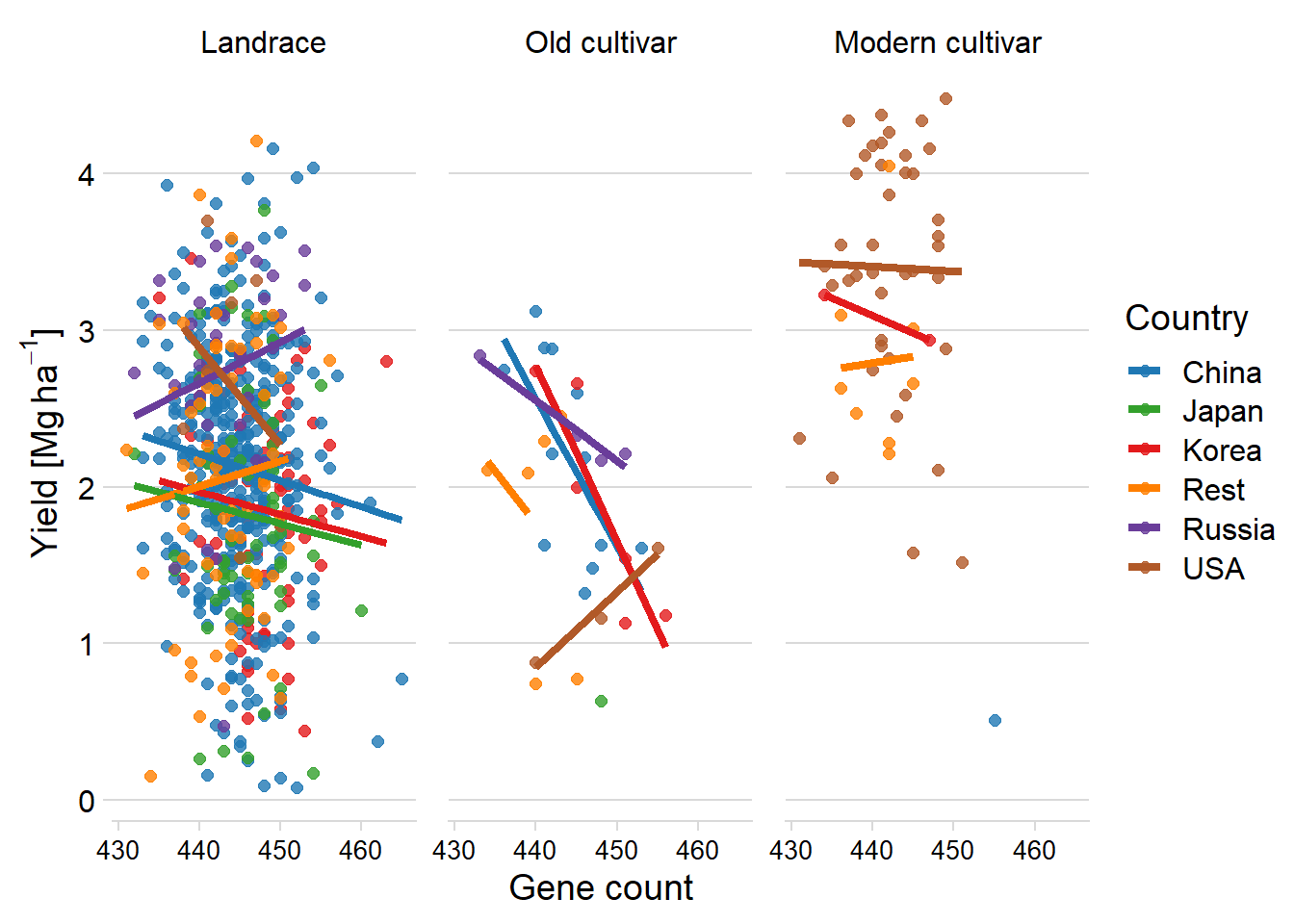

six_country_table %>% filter(Country2 == 'China') %>% 
  add_predictions(models$China) %>% 
  ggplot(aes(x = Count, y = pred, color = Country2)) +
  facet_wrap(~ Group, nrow = 1) +  
  geom_point(aes(y = Yield, color = Country2),
    alpha = 0.8,
    size = 2) +
  geom_line(aes(y=pred, group=interaction(Group, Country),colour=Country2), size=1.5)+
  theme_minimal_hgrid() +
  xlab('Gene count') +
  ylab(expression(paste('Yield [Mg ', ha ^ -1, ']'))) +
  scale_color_manual(values = mycol) +
  #xlim(c(47.900, 49.700)) +
  labs(color = "Country") +
  theme(panel.spacing = unit(0.9, "lines"),
  axis.text.x = element_text(size = 10))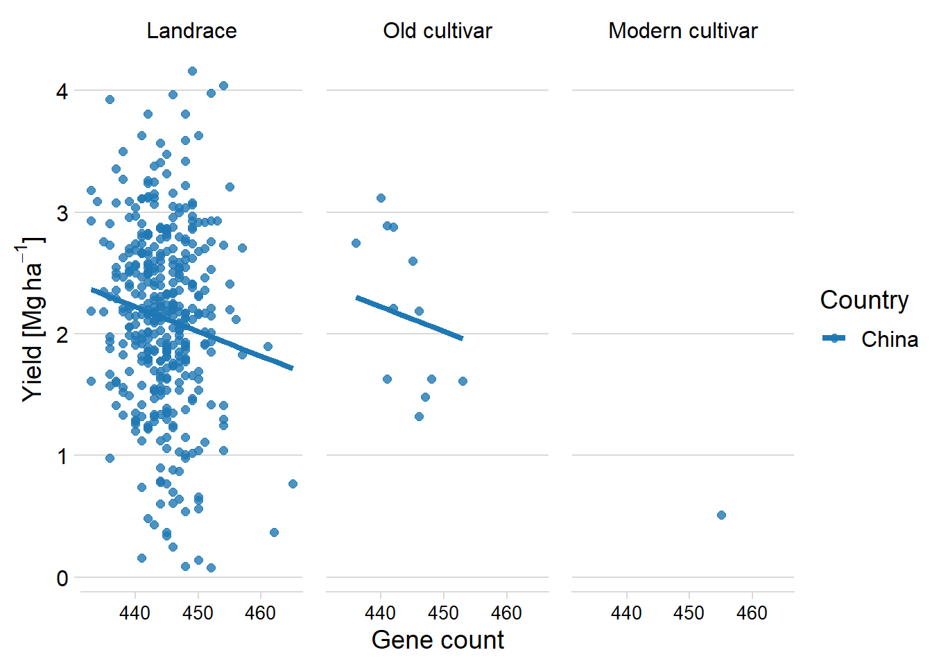

six_country_table %>% filter(Country2 == 'USA') %>% 
  add_predictions(models$USA) %>% 
  ggplot(aes(x = Count, y = pred, color = Country2)) +
  facet_wrap(~ Group, nrow = 1) +  
  geom_point(aes(y = Yield, color = Country2),
    alpha = 0.8,
    size = 2) +
  geom_line(aes(y=pred, group=interaction(Group, Country),colour=Country2), size=1.5)+
  theme_minimal_hgrid() +
  xlab('Gene count') +
  ylab(expression(paste('Yield [Mg ', ha ^ -1, ']'))) +
  scale_color_manual(values = mycol) +
  #xlim(c(47.900, 49.700)) +
  labs(color = "Country") +
  theme(panel.spacing = unit(0.9, "lines"),
  axis.text.x = element_text(size = 10))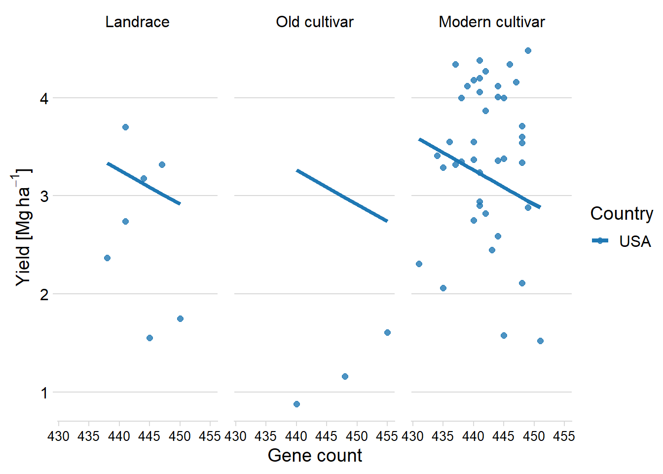

single_model <- lm(Yield ~ Count+Group, data = six_country_table)

plot_model(single_model, show.values = TRUE,)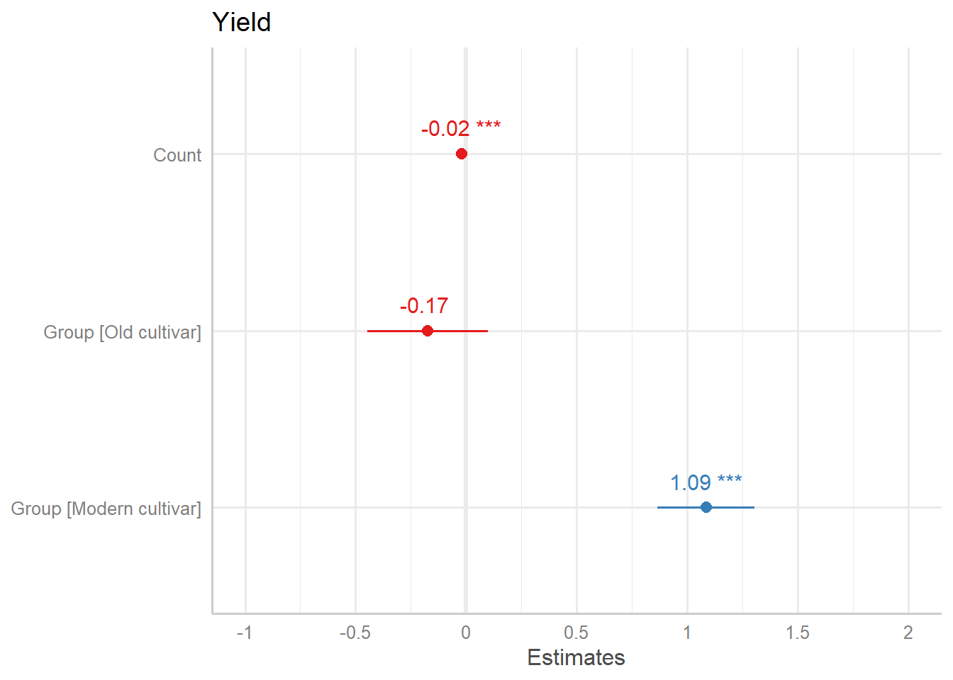

six_country_table %>% 
  add_predictions(single_model) %>% 
  ggplot(aes(x = Count, y = pred)) +
  facet_wrap(~ Group, nrow = 1) +  
  geom_point(aes(y = Yield),
    alpha = 0.8,
    size = 2) +
  geom_line(aes(y=pred, group=interaction(Group, Country)), size=1.5)+
  theme_minimal_hgrid() +
  xlab('Gene count') +
  ylab(expression(paste('Yield [Mg ', ha ^ -1, ']'))) +
  scale_color_manual(values = mycol) +
  #xlim(c(47.900, 49.700)) +
  labs(color = "Country") +
  theme(panel.spacing = unit(0.9, "lines"),
  axis.text.x = element_text(size = 10))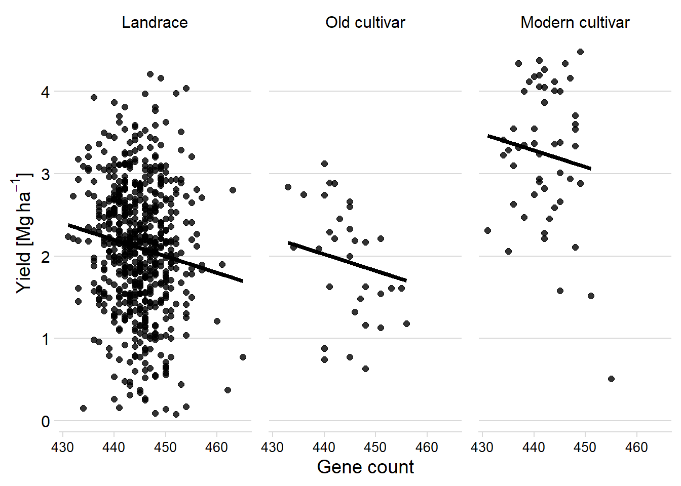

FINALLY, let’s make one model per breeding group:

mymodel <-  function(df) { lm(Yield ~ Count, data=df) }

results <- six_country_table %>% nest(data = -c(Group)) %>% 
  mutate(model = map(data, mymodel)) %>% 
  mutate(pred = map2(data, model, add_predictions))

results %>% 
  unnest(pred) %>% 
  select(-c(data, model)) %>% 
  ggplot(aes(x = Count, y = pred, color=Group)) +
  facet_wrap(~ Group, nrow = 1) +  
  geom_point(aes(y = Yield),
    alpha = 0.8,
    size = 2) +
  geom_line(aes(y=pred, group=interaction(Group, Country)), size=1.5)+
  theme_minimal_hgrid() +
  xlab('Gene count') +
  ylab(expression(paste('Yield [Mg ', ha ^ -1, ']'))) +
  scale_color_manual(values = mycol) +
  #xlim(c(47.900, 49.700)) +
  labs(color = "Country") +
  theme(panel.spacing = unit(0.9, "lines"),
  axis.text.x = element_text(size = 10))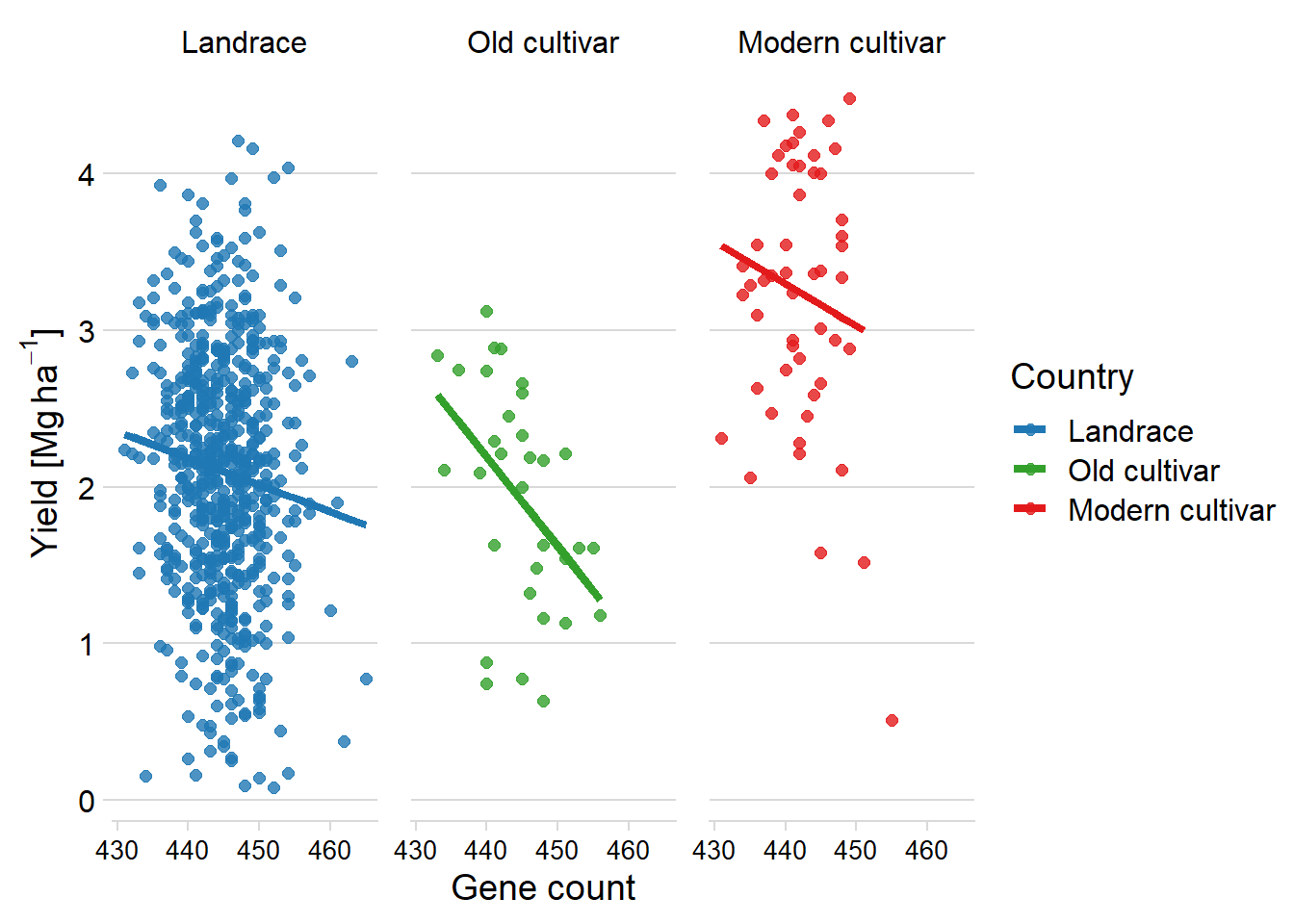

plot_models(results$model, m.labels = results$Group, p.shape=TRUE) +
  scale_colour_manual(values = mycol)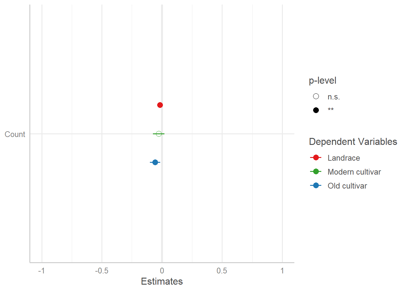

As a last check - what happens if I remove outliers from the moderns, do I then get an association?

results <- six_country_table %>% filter(!(Group == 'Modern cultivar' & Yield < 2)) %>% 
  nest(data = -c(Group)) %>% 
  mutate(model = map(data, mymodel)) %>% 
  mutate(pred = map2(data, model, add_predictions))


results %>% 
  unnest(pred) %>% 
  select(-c(data, model)) %>% 
  ggplot(aes(x = Count, y = pred, color=Group)) +
  facet_wrap(~ Group, nrow = 1) +  
  geom_point(aes(y = Yield),
    alpha = 0.8,
    size = 2) +
  geom_line(aes(y=pred, group=interaction(Group, Country)), size=1.5)+
  theme_minimal_hgrid() +
  xlab('Gene count') +
  ylab(expression(paste('Yield [Mg ', ha ^ -1, ']'))) +
  scale_color_manual(values = mycol) +
  #xlim(c(47.900, 49.700)) +
  labs(color = "Country") +
  theme(panel.spacing = unit(0.9, "lines"),
  axis.text.x = element_text(size = 10))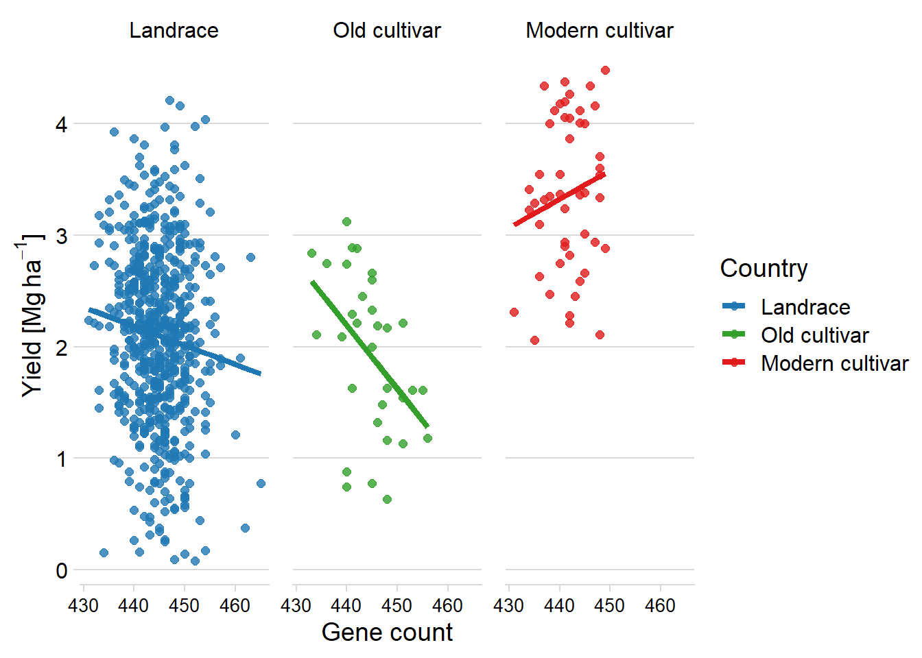

plot_models(results$model, m.labels = results$Group, p.shape=TRUE) +
  scale_colour_manual(values = mycol)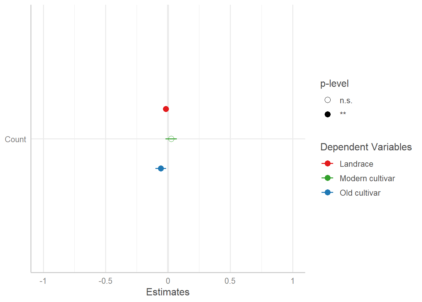

results <- six_country_table %>% filter(Group == 'Modern cultivar' & Yield >2) %>% 
  nest(data = -c(Group)) %>% 
  mutate(model = map(data, mymodel)) %>% 
  mutate(pred = map2(data, model, add_predictions))


results %>% 
  unnest(pred) %>% 
  select(-c(data, model)) %>% 
  ggplot(aes(x = Count, y = pred, color=Group)) +
  facet_wrap(~ Group, nrow = 1) +  
  geom_point(aes(y = Yield),
    alpha = 0.8,
    size = 2) +
  geom_line(aes(y=pred, group=interaction(Group, Country)), size=1.5)+
  theme_minimal_hgrid() +
  xlab('Gene count') +
  ylab(expression(paste('Yield [Mg ', ha ^ -1, ']'))) +
  scale_color_manual(values = mycol) +
  #xlim(c(47.900, 49.700)) +
  labs(color = "Country") +
  theme(panel.spacing = unit(0.9, "lines"),
  axis.text.x = element_text(size = 10))

Protein

protein_nbs_joined_groups <- nbs_joined_groups %>% inner_join(protein_join, by = 'names') 
#protein_nbs_joined_groups$Protein2 <- scale(protein_nbs_joined_groups$Protein, center=T, scale=T)
protein_country_nbs_joined_groups <- protein_nbs_joined_groups %>% inner_join(country)
#protein_country_nbs_joined_groups <- rename(protein_country_nbs_joined_groups, Group=`Group in violin table`)
protein_country_nbs_joined_groups <- protein_country_nbs_joined_groups %>% filter(Group != 'Wild')
protein_country_nbs_joined_groups <- protein_country_nbs_joined_groups %>% rename(Count = presences.x)

lm_model <- lm(Protein ~ Count +  Group, data = protein_country_nbs_joined_groups) 
summary(lm_model)


Call:
lm(formula = Protein ~ Count + Group, data = protein_country_nbs_joined_groups)

Residuals:
    Min      1Q  Median      3Q     Max 
-7.4693 -1.9952 -0.1035  1.6965  9.5650 

Coefficients:
                     Estimate Std. Error t value Pr(>|t|)    
(Intercept)          29.16057    8.99723   3.241 0.001241 ** 
Count                 0.03425    0.02023   1.693 0.090781 .  
GroupOld cultivar    -1.53490    0.45402  -3.381 0.000759 ***
GroupModern cultivar -1.42768    0.35601  -4.010 6.64e-05 ***
---
Signif. codes:  0 '***' 0.001 '**' 0.01 '*' 0.05 '.' 0.1 ' ' 1

Residual standard error: 2.823 on 785 degrees of freedom
Multiple R-squared:  0.03787,   Adjusted R-squared:  0.0342 
F-statistic:  10.3 on 3 and 785 DF,  p-value: 1.178e-06

clm_model <- lm(Protein ~ Count +  Group + Country, data = protein_country_nbs_joined_groups) 
summary(clm_model)


Call:
lm(formula = Protein ~ Count + Group + Country, data = protein_country_nbs_joined_groups)

Residuals:
    Min      1Q  Median      3Q     Max 
-7.5543 -1.8497 -0.1008  1.6682  9.9914 

Coefficients:
                     Estimate Std. Error t value Pr(>|t|)    
(Intercept)          37.14499    9.50557   3.908 0.000102 ***
Count                 0.01416    0.02121   0.668 0.504547    
GroupOld cultivar    -1.59216    0.47823  -3.329 0.000914 ***
GroupModern cultivar -0.83999    0.76763  -1.094 0.274196    
CountryArgentina      0.17776    2.65850   0.067 0.946708    
CountryAustralia      0.88155    2.54745   0.346 0.729403    
CountryAustria       -1.70472    3.21970  -0.529 0.596642    
CountryBelgium        0.50944    2.54543   0.200 0.841426    
CountryBrazil         0.36257    2.13865   0.170 0.865423    
CountryBulgaria      -0.94807    3.22063  -0.294 0.768554    
CountryCanada        -0.53675    2.00875  -0.267 0.789386    
CountryChina          1.02128    1.61681   0.632 0.527801    
CountryCosta Rica    -2.54807    3.22063  -0.791 0.429098    
CountryFormer Serbia  0.83527    3.31001   0.252 0.800843    
CountryFrance        -0.95096    2.12998  -0.446 0.655392    
CountryGeorgia        0.79485    2.54627   0.312 0.755007    
CountryGermany       -0.31615    2.14375  -0.147 0.882795    
CountryHungary       -0.51513    2.13047  -0.242 0.809010    
CountryIndia          1.49958    1.89230   0.792 0.428346    
CountryIndonesia      3.23487    2.13047   1.518 0.129347    
CountryItaly          0.47328    3.25514   0.145 0.884440    
CountryJapan          0.31111    1.64568   0.189 0.850108    
CountryKorea          2.11269    1.64371   1.285 0.199087    
CountryKyrgyzstan    -2.50472    3.21970  -0.778 0.436856    
CountryMoldova       -1.24935    1.92485  -0.649 0.516498    
CountryMorocco        2.79701    3.23401   0.865 0.387390    
CountryMyanmar        5.79442    2.54931   2.273 0.023318 *  
CountryNepal          0.52404    2.54568   0.206 0.836963    
CountryNetherlands   -1.79056    3.21972  -0.556 0.578296    
CountryPakistan      -1.99142    3.22379  -0.618 0.536947    
CountryPeru           2.06695    3.22007   0.642 0.521139    
CountryPoland         0.12447    3.22167   0.039 0.969192    
CountryRomania       -1.91888    1.97185  -0.973 0.330804    
CountryRussia         1.14427    1.67007   0.685 0.493458    
CountrySerbia        -1.11888    2.54554  -0.440 0.660395    
CountrySouth Africa  -1.90808    3.31005  -0.576 0.564487    
CountrySweden        -0.68287    2.28541  -0.299 0.765181    
CountryTaiwan         2.00539    2.03916   0.983 0.325715    
CountryTanzania      -2.96137    3.22100  -0.919 0.358190    
CountryUkraine       -2.44721    3.22046  -0.760 0.447562    
CountryUSA            0.37499    1.76882   0.212 0.832164    
CountryUzbekistan    -2.43391    3.22121  -0.756 0.450137    
CountryVietnam        2.17404    2.12998   1.021 0.307739    
---
Signif. codes:  0 '***' 0.001 '**' 0.01 '*' 0.05 '.' 0.1 ' ' 1

Residual standard error: 2.788 on 736 degrees of freedom
  (10 observations deleted due to missingness)
Multiple R-squared:  0.112, Adjusted R-squared:  0.06128 
F-statistic: 2.209 on 42 and 736 DF,  p-value: 2.577e-05

protmod <- clm_model

Seed weight

seed_nbs_joined_groups <- nbs_joined_groups %>% inner_join(seed_join, by = 'names') 
#seed_nbs_joined_groups$wt2 <- scale(seed_nbs_joined_groups$wt, center=T, scale=T)
seed_country_nbs_joined_groups <- seed_nbs_joined_groups %>% inner_join(country)
#seed_country_nbs_joined_groups <- rename(seed_country_nbs_joined_groups, Group = `Group in violin table`)
seed_country_nbs_joined_groups <- seed_country_nbs_joined_groups %>% filter(Group != 'Wild')
seed_country_nbs_joined_groups <- seed_country_nbs_joined_groups %>% rename(Count = presences.x)

lm_model <- lm(wt ~ Count +  Group, data = seed_country_nbs_joined_groups) 
summary(lm_model)


Call:
lm(formula = wt ~ Count + Group, data = seed_country_nbs_joined_groups)

Residuals:
     Min       1Q   Median       3Q      Max 
-11.0968  -2.7970   0.0037   2.5611  19.6026 

Coefficients:
                      Estimate Std. Error t value Pr(>|t|)   
(Intercept)          1.314e+01  1.512e+01   0.869  0.38510   
Count                1.307e-04  3.399e-02   0.004  0.99693   
GroupOld cultivar    1.612e+00  7.732e-01   2.085  0.03745 * 
GroupModern cultivar 1.643e+00  6.035e-01   2.723  0.00665 **
---
Signif. codes:  0 '***' 0.001 '**' 0.01 '*' 0.05 '.' 0.1 ' ' 1

Residual standard error: 4.188 on 629 degrees of freedom
Multiple R-squared:  0.01745,   Adjusted R-squared:  0.01276 
F-statistic: 3.724 on 3 and 629 DF,  p-value: 0.01129

clm_model <- lm(wt ~ Count +  Group + Country, data = seed_country_nbs_joined_groups) 
summary(clm_model)


Call:
lm(formula = wt ~ Count + Group + Country, data = seed_country_nbs_joined_groups)

Residuals:
    Min      1Q  Median      3Q     Max 
-12.222  -2.473   0.000   2.297  19.312 

Coefficients:
                     Estimate Std. Error t value Pr(>|t|)    
(Intercept)          20.41722   15.96470   1.279 0.201439    
Count                -0.02562    0.03574  -0.717 0.473706    
GroupOld cultivar     1.01558    0.84334   1.204 0.228982    
GroupModern cultivar  1.78999    1.32483   1.351 0.177182    
CountryArgentina      1.16481    4.94786   0.235 0.813967    
CountryAustralia      5.32385    3.77255   1.411 0.158714    
CountryBelgium        4.03167    4.76789   0.846 0.398127    
CountryBrazil         4.05979    3.37177   1.204 0.229054    
CountryBulgaria       4.40605    4.76874   0.924 0.355895    
CountryCanada         4.83881    3.21326   1.506 0.132634    
CountryChina          3.97326    2.39648   1.658 0.097861 .  
CountryCosta Rica     4.60605    4.76874   0.966 0.334500    
CountryFormer Serbia  5.61855    4.94786   1.136 0.256607    
CountryFrance        13.55072    3.77898   3.586 0.000364 ***
CountryGeorgia        7.51886    3.77029   1.994 0.046588 *  
CountryGermany        8.35203    3.86586   2.160 0.031141 *  
CountryHungary        6.85125    3.37149   2.032 0.042592 *  
CountryIndia         -0.33772    3.02336  -0.112 0.911098    
CountryIndonesia     -0.11542    3.37149  -0.034 0.972702    
CountryItaly          1.81858    4.84127   0.376 0.707319    
CountryJapan          5.17895    2.44293   2.120 0.034427 *  
CountryKorea          4.44772    2.44494   1.819 0.069397 .  
CountryKyrgyzstan     4.80854    4.76695   1.009 0.313522    
CountryMoldova        2.58441    3.01551   0.857 0.391773    
CountryMorocco        7.26728    4.79439   1.516 0.130111    
CountryMyanmar       -1.57083    3.77612  -0.416 0.677570    
CountryNepal          3.14698    3.76916   0.835 0.404099    
CountryPakistan      -4.99645    4.77481  -1.046 0.295798    
CountryPeru           7.45979    4.76767   1.565 0.118201    
CountryRomania        3.53479    3.15414   1.121 0.262881    
CountryRussia         4.72218    2.48399   1.901 0.057785 .  
CountrySerbia         2.13417    3.76890   0.566 0.571435    
CountrySouth Africa   2.71606    4.94682   0.549 0.583179    
CountrySweden         8.10668    3.38864   2.392 0.017056 *  
CountryTaiwan         3.89395    3.37328   1.154 0.248826    
CountryTanzania       5.01104    4.76945   1.051 0.293851    
CountryUkraine        9.08541    4.76843   1.905 0.057226 .  
CountryUSA            3.91751    2.69217   1.455 0.146162    
CountryUzbekistan     5.28042    4.76985   1.107 0.268730    
CountryVietnam       -0.22802    3.15371  -0.072 0.942385    
---
Signif. codes:  0 '***' 0.001 '**' 0.01 '*' 0.05 '.' 0.1 ' ' 1

Residual standard error: 4.128 on 587 degrees of freedom
  (6 observations deleted due to missingness)
Multiple R-squared:  0.09879,   Adjusted R-squared:  0.03892 
F-statistic:  1.65 on 39 and 587 DF,  p-value: 0.008891

seedmod <- clm_model

Nothing at all.

Oil content

oil_nbs_joined_groups <- nbs_joined_groups %>% inner_join(oil_join, by = 'names') 
oil_nbs_joined_groups$Oil2 <- scale(oil_nbs_joined_groups$Oil, center=T, scale=T)
oil_country_nbs_joined_groups <- oil_nbs_joined_groups %>% inner_join(country)
oil_country_nbs_joined_groups <- oil_country_nbs_joined_groups %>% filter(Group != 'Wild')
oil_country_nbs_joined_groups <- oil_country_nbs_joined_groups %>% rename(Count = presences.x)

lm_model <- lm(Oil ~ Count +  Group, data = oil_country_nbs_joined_groups) 
summary(lm_model)


Call:
lm(formula = Oil ~ Count + Group, data = oil_country_nbs_joined_groups)

Residuals:
     Min       1Q   Median       3Q      Max 
-10.0707  -1.2772   0.2899   1.5654   7.0260 

Coefficients:
                     Estimate Std. Error t value Pr(>|t|)    
(Intercept)          35.58518    7.29827   4.876 1.31e-06 ***
Count                -0.03935    0.01641  -2.398  0.01671 *  
GroupOld cultivar     1.17018    0.36829   3.177  0.00154 ** 
GroupModern cultivar  1.77380    0.28878   6.142 1.29e-09 ***
---
Signif. codes:  0 '***' 0.001 '**' 0.01 '*' 0.05 '.' 0.1 ' ' 1

Residual standard error: 2.29 on 785 degrees of freedom
Multiple R-squared:  0.06684,   Adjusted R-squared:  0.06328 
F-statistic: 18.74 on 3 and 785 DF,  p-value: 9.485e-12

Interesting, the simple model has p< 0.05 for oil content!

clm_model <- lm(Oil ~ Count +  Group + Country, data = oil_country_nbs_joined_groups) 
summary(clm_model)


Call:
lm(formula = Oil ~ Count + Group + Country, data = oil_country_nbs_joined_groups)

Residuals:
    Min      1Q  Median      3Q     Max 
-9.8810 -1.2328  0.1494  1.4493  6.9085 

Coefficients:
                     Estimate Std. Error t value Pr(>|t|)    
(Intercept)          29.54369    7.66209   3.856 0.000125 ***
Count                -0.02893    0.01710  -1.692 0.091068 .  
GroupOld cultivar     1.04686    0.38549   2.716 0.006769 ** 
GroupModern cultivar  1.27422    0.61876   2.059 0.039816 *  
CountryArgentina      2.43197    2.14292   1.135 0.256792    
CountryAustralia      2.17316    2.05341   1.058 0.290257    
CountryAustria        2.64298    2.59528   1.018 0.308832    
CountryBelgium        1.31405    2.05177   0.640 0.522083    
CountryBrazil         2.11058    1.72389   1.224 0.221224    
CountryBulgaria       1.62726    2.59603   0.627 0.530967    
CountryCanada         2.82941    1.61918   1.747 0.080979 .  
CountryChina          1.52124    1.30325   1.167 0.243480    
CountryCosta Rica     3.52726    2.59603   1.359 0.174654    
CountryFormer Serbia  3.06876    2.66808   1.150 0.250445    
CountryFrance         2.91137    1.71690   1.696 0.090363 .  
CountryGeorgia        0.94172    2.05246   0.459 0.646493    
CountryGermany        2.73276    1.72799   1.581 0.114202    
CountryHungary        3.59030    1.71729   2.091 0.036900 *  
CountryIndia         -1.39957    1.52531  -0.918 0.359149    
CountryIndonesia     -0.48470    1.71729  -0.282 0.777834    
CountryItaly          2.92505    2.62385   1.115 0.265303    
CountryJapan          1.26616    1.32653   0.954 0.340149    
CountryKorea          0.69858    1.32494   0.527 0.598176    
CountryKyrgyzstan     2.74298    2.59528   1.057 0.290899    
CountryMoldova        2.23354    1.55155   1.440 0.150419    
CountryMorocco        2.54798    2.60682   0.977 0.328677    
CountryMyanmar       -1.90953    2.05491  -0.929 0.353063    
CountryNepal          1.33637    2.05198   0.651 0.515083    
CountryNetherlands    1.81405    2.59530   0.699 0.484788    
CountryPakistan      -4.38846    2.59858  -1.689 0.091683 .  
CountryPeru          -0.89917    2.59558  -0.346 0.729125    
CountryPoland         3.68762    2.59687   1.420 0.156024    
CountryRomania        2.70524    1.58944   1.702 0.089175 .  
CountryRussia         1.59189    1.34619   1.183 0.237382    
CountrySerbia         2.17191    2.05187   1.059 0.290174    
CountrySouth Africa   3.75304    2.66811   1.407 0.159959    
CountrySweden         2.41498    1.84218   1.311 0.190289    
CountryTaiwan         0.65146    1.64369   0.396 0.691968    
CountryTanzania       5.85869    2.59633   2.257 0.024330 *  
CountryUkraine        3.32976    2.59590   1.283 0.200000    
CountryUSA            1.79837    1.42578   1.261 0.207592    
CountryUzbekistan     2.29833    2.59650   0.885 0.376356    
CountryVietnam       -1.51363    1.71690  -0.882 0.378277    
---
Signif. codes:  0 '***' 0.001 '**' 0.01 '*' 0.05 '.' 0.1 ' ' 1

Residual standard error: 2.248 on 736 degrees of freedom
  (10 observations deleted due to missingness)
Multiple R-squared:  0.148, Adjusted R-squared:  0.09939 
F-statistic: 3.044 on 42 and 736 DF,  p-value: 1.373e-09

oilmod <- clm_model

p = 0.07 for Count + Group + Country in the model

All models together

tab_model(yieldmod, oilmod, protmod, seedmod, digits=3 )

	Yield			Oil			Protein			wt
Predictors	Estimates	CI	p	Estimates	CI	p	Estimates	CI	p	Estimates	CI	p
(Intercept)	9.307	4.295 – 14.318	<0.001	29.544	14.502 – 44.586	<0.001	37.145	18.484 – 55.806	<0.001	20.417	-10.938 – 51.772	0.201
Count	-0.016	-0.027 – -0.005	0.005	-0.029	-0.062 – 0.005	0.091	0.014	-0.027 – 0.056	0.505	-0.026	-0.096 – 0.045	0.474
Group [Old cultivar]	-0.218	-0.491 – 0.056	0.118	1.047	0.290 – 1.804	0.007	-1.592	-2.531 – -0.653	0.001	1.016	-0.641 – 2.672	0.229
Group [Modern cultivar]	0.801	0.380 – 1.222	<0.001	1.274	0.059 – 2.489	0.040	-0.840	-2.347 – 0.667	0.274	1.790	-0.812 – 4.392	0.177
Country [Argentina]	-0.599	-1.961 – 0.763	0.388	2.432	-1.775 – 6.639	0.257	0.178	-5.041 – 5.397	0.947	1.165	-8.553 – 10.882	0.814
Country [Australia]	-0.684	-2.323 – 0.955	0.413	2.173	-1.858 – 6.204	0.290	0.882	-4.120 – 5.883	0.729	5.324	-2.085 – 12.733	0.159
Country [Austria]	0.415	-1.223 – 2.053	0.619	2.643	-2.452 – 7.738	0.309	-1.705	-8.026 – 4.616	0.597
Country [Belgium]	-0.291	-1.586 – 1.004	0.660	1.314	-2.714 – 5.342	0.522	0.509	-4.488 – 5.507	0.841	4.032	-5.333 – 13.396	0.398
Country [Brazil]	-0.734	-2.373 – 0.905	0.379	2.111	-1.274 – 5.495	0.221	0.363	-3.836 – 4.561	0.865	4.060	-2.562 – 10.682	0.229
Country [Bulgaria]	-0.419	-2.057 – 1.220	0.616	1.627	-3.469 – 6.724	0.531	-0.948	-7.271 – 5.375	0.769	4.406	-4.960 – 13.772	0.356
Country [Canada]	-0.151	-1.245 – 0.943	0.786	2.829	-0.349 – 6.008	0.081	-0.537	-4.480 – 3.407	0.789	4.839	-1.472 – 11.150	0.133
Country [China]	-0.028	-0.851 – 0.794	0.946	1.521	-1.037 – 4.080	0.243	1.021	-2.153 – 4.195	0.528	3.973	-0.733 – 8.680	0.098
Country [Costa Rica]	0.781	-0.857 – 2.420	0.350	3.527	-1.569 – 8.624	0.175	-2.548	-8.871 – 3.775	0.429	4.606	-4.760 – 13.972	0.335
Country [Former Serbia]	1.044	-0.647 – 2.736	0.226	3.069	-2.169 – 8.307	0.250	0.835	-5.663 – 7.333	0.801	5.619	-4.099 – 15.336	0.257
Country [France]	0.309	-0.774 – 1.393	0.575	2.911	-0.459 – 6.282	0.090	-0.951	-5.133 – 3.231	0.655	13.551	6.129 – 20.973	<0.001
Country [Georgia]	0.814	-0.481 – 2.110	0.218	0.942	-3.088 – 4.971	0.646	0.795	-4.204 – 5.794	0.755	7.519	0.114 – 14.924	0.047
Country [Germany]	-0.241	-1.334 – 0.851	0.664	2.733	-0.660 – 6.125	0.114	-0.316	-4.525 – 3.892	0.883	8.352	0.759 – 15.945	0.031
Country [Hungary]	0.613	-0.471 – 1.697	0.267	3.590	0.219 – 6.962	0.037	-0.515	-4.698 – 3.667	0.809	6.851	0.230 – 13.473	0.043
Country [India]	-1.154	-2.239 – -0.070	0.037	-1.400	-4.394 – 1.595	0.359	1.500	-2.215 – 5.215	0.428	-0.338	-6.276 – 5.600	0.911
Country [Indonesia]	-1.244	-2.328 – -0.161	0.024	-0.485	-3.856 – 2.887	0.778	3.235	-0.948 – 7.417	0.129	-0.115	-6.737 – 6.506	0.973
Country [Italy]	0.479	-1.182 – 2.140	0.571	2.925	-2.226 – 8.076	0.265	0.473	-5.917 – 6.864	0.884	1.819	-7.690 – 11.327	0.707
Country [Japan]	-0.336	-1.174 – 0.503	0.432	1.266	-1.338 – 3.870	0.340	0.311	-2.920 – 3.542	0.850	5.179	0.381 – 9.977	0.034
Country [Korea]	-0.230	-1.067 – 0.606	0.589	0.699	-1.903 – 3.300	0.598	2.113	-1.114 – 5.340	0.199	4.448	-0.354 – 9.250	0.069
Country [Kyrgyzstan]	0.705	-0.933 – 2.343	0.398	2.743	-2.352 – 7.838	0.291	-2.505	-8.826 – 3.816	0.437	4.809	-4.554 – 14.171	0.314
Country [Moldova]	0.021	-0.958 – 1.001	0.966	2.234	-0.812 – 5.280	0.150	-1.249	-5.028 – 2.529	0.516	2.584	-3.338 – 8.507	0.392
Country [Morocco]	0.830	-0.816 – 2.476	0.322	2.548	-2.570 – 7.666	0.329	2.797	-3.552 – 9.146	0.387	7.267	-2.149 – 16.684	0.130
Country [Myanmar]	-1.112	-2.409 – 0.185	0.093	-1.910	-5.944 – 2.125	0.353	5.794	0.790 – 10.799	0.023	-1.571	-8.987 – 5.846	0.678
Country [Nepal]	-0.446	-1.741 – 0.850	0.500	1.336	-2.692 – 5.365	0.515	0.524	-4.474 – 5.522	0.837	3.147	-4.256 – 10.550	0.404
Country [Netherlands]	-0.711	-2.349 – 0.927	0.395	1.814	-3.281 – 6.909	0.485	-1.791	-8.111 – 4.530	0.578
Country [Pakistan]	-2.183	-3.823 – -0.543	0.009	-4.388	-9.490 – 0.713	0.092	-1.991	-8.320 – 4.338	0.537	-4.996	-14.374 – 4.381	0.296
Country [Peru]	-1.183	-2.821 – 0.456	0.157	-0.899	-5.995 – 4.196	0.729	2.067	-4.255 – 8.389	0.521	7.460	-1.904 – 16.824	0.118
Country [Poland]	0.956	-0.683 – 2.595	0.253	3.688	-1.411 – 8.786	0.156	0.124	-6.200 – 6.449	0.969
Country [Romania]	1.153	0.150 – 2.156	0.024	2.705	-0.415 – 5.826	0.089	-1.919	-5.790 – 1.952	0.331	3.535	-2.660 – 9.730	0.263
Country [Russia]	0.540	-0.310 – 1.389	0.213	1.592	-1.051 – 4.235	0.237	1.144	-2.134 – 4.423	0.493	4.722	-0.156 – 9.601	0.058
Country [Serbia]	0.221	-1.074 – 1.516	0.737	2.172	-1.856 – 6.200	0.290	-1.119	-6.116 – 3.879	0.660	2.134	-5.268 – 9.536	0.571
Country [South Africa]	-0.600	-2.291 – 1.091	0.486	3.753	-1.485 – 8.991	0.160	-1.908	-8.406 – 4.590	0.564	2.716	-7.000 – 12.432	0.583
Country [Sweden]	-0.766	-1.930 – 0.397	0.196	2.415	-1.202 – 6.032	0.190	-0.683	-5.170 – 3.804	0.765	8.107	1.451 – 14.762	0.017
Country [Taiwan]	-0.657	-1.695 – 0.381	0.214	0.651	-2.575 – 3.878	0.692	2.005	-1.998 – 6.009	0.326	3.894	-2.731 – 10.519	0.249
Country [Ukraine]	0.724	-0.915 – 2.362	0.386	3.330	-1.766 – 8.426	0.200	-2.447	-8.770 – 3.875	0.448	9.085	-0.280 – 18.451	0.057
Country [USA]	0.346	-0.564 – 1.256	0.456	1.798	-1.001 – 4.597	0.208	0.375	-3.098 – 3.848	0.832	3.918	-1.370 – 9.205	0.146
Country [Uzbekistan]	0.315	-1.324 – 1.954	0.706	2.298	-2.799 – 7.396	0.376	-2.434	-8.758 – 3.890	0.450	5.280	-4.088 – 14.648	0.269
Country [Vietnam]	-0.693	-1.777 – 0.391	0.210	-1.514	-4.884 – 1.857	0.378	2.174	-2.008 – 6.356	0.308	-0.228	-6.422 – 5.966	0.942
Country [Tanzania]				5.859	0.762 – 10.956	0.024	-2.961	-9.285 – 3.362	0.358	5.011	-4.356 – 14.378	0.294
Observations	731			779			779			627
R² / R² adjusted	0.283 / 0.240			0.148 / 0.099			0.112 / 0.061			0.099 / 0.039

The yield model for all genes

yield_country_all_joined_groups <- yield_country_all_joined_groups %>% dplyr::rename(`All genes` = presences.x)

clm <- lm(Yield ~ `All genes` + Group + Country, data=yield_country_all_joined_groups)
summary(clm)


Call:
lm(formula = Yield ~ `All genes` + Group + Country, data = yield_country_all_joined_groups)

Residuals:
     Min       1Q   Median       3Q      Max 
-2.45433 -0.38016  0.01363  0.45362  2.01898 

Coefficients:
                       Estimate Std. Error t value Pr(>|t|)    
(Intercept)           4.3846649  9.4830523   0.462 0.643963    
`All genes`          -0.0000450  0.0001961  -0.230 0.818513    
GroupOld cultivar    -0.2181643  0.1401041  -1.557 0.119892    
GroupModern cultivar  0.8284865  0.2171747   3.815 0.000149 ***
CountryArgentina     -0.5842141  0.6978474  -0.837 0.402790    
CountryAustralia     -0.7716951  0.8390702  -0.920 0.358050    
CountryAustria        0.4071798  0.8391277   0.485 0.627659    
CountryBelgium       -0.2806376  0.6633234  -0.423 0.672370    
CountryBrazil        -0.8234953  0.8391759  -0.981 0.326782    
CountryBulgaria      -0.3590849  0.8390472  -0.428 0.668809    
CountryCanada        -0.1765815  0.5604944  -0.315 0.752822    
CountryChina         -0.0722465  0.4211295  -0.172 0.863838    
CountryCosta Rica     0.8302041  0.8401223   0.988 0.323404    
CountryFormer Serbia  1.0045079  0.8662586   1.160 0.246616    
CountryFrance         0.2812639  0.5549986   0.507 0.612469    
CountryGeorgia        0.8601321  0.6636565   1.296 0.195392    
CountryGermany       -0.1990329  0.5593739  -0.356 0.722089    
CountryHungary        0.5695627  0.5550440   1.026 0.305177    
CountryIndia         -1.2192424  0.5549811  -2.197 0.028359 *  
CountryIndonesia     -1.2874198  0.5550851  -2.319 0.020669 *  
CountryItaly          0.4669101  0.8516478   0.548 0.583703    
CountryJapan         -0.3986662  0.4288991  -0.930 0.352950    
CountryKorea         -0.3196161  0.4275551  -0.748 0.454990    
CountryKyrgyzstan     0.6991149  0.8390466   0.833 0.405006    
CountryMoldova       -0.0165313  0.5014997  -0.033 0.973713    
CountryMorocco        0.6192767  0.8432298   0.734 0.462949    
CountryMyanmar       -1.0069877  0.6633741  -1.518 0.129478    
CountryNepal         -0.4759751  0.6633311  -0.718 0.473276    
CountryNetherlands   -0.7048454  0.8393032  -0.840 0.401313    
CountryPakistan      -2.0554396  0.8392729  -2.449 0.014571 *  
CountryPeru          -1.2263756  0.8394973  -1.461 0.144514    
CountryPoland         0.8733453  0.8391643   1.041 0.298365    
CountryRomania        1.1384698  0.5146576   2.212 0.027288 *  
CountryRussia         0.5181480  0.4352209   1.191 0.234244    
CountrySerbia         0.1960997  0.6635351   0.296 0.767672    
CountrySouth Africa  -0.5749971  0.8662537  -0.664 0.507057    
CountrySweden        -0.8583437  0.5951344  -1.442 0.149681    
CountryTaiwan        -0.6960443  0.5314349  -1.310 0.190719    
CountryUkraine        0.6639845  0.8394469   0.791 0.429229    
CountryUSA            0.3072519  0.4662389   0.659 0.510115    
CountryUzbekistan     0.3874948  0.8391087   0.462 0.644375    
CountryVietnam       -0.7200660  0.5550726  -1.297 0.194981    
---
Signif. codes:  0 '***' 0.001 '**' 0.01 '*' 0.05 '.' 0.1 ' ' 1

Residual standard error: 0.7266 on 689 degrees of freedom
  (10 observations deleted due to missingness)
Multiple R-squared:  0.2747,    Adjusted R-squared:  0.2316 
F-statistic: 6.365 on 41 and 689 DF,  p-value: < 2.2e-16

Good, p > 0.05

Let’s try the model without group and country

baselm <- lm(as.numeric(Group) ~ `All genes`, data=yield_country_all_joined_groups)
summary(baselm)


Call:
lm(formula = as.numeric(Group) ~ `All genes`, data = yield_country_all_joined_groups)

Residuals:
    Min      1Q  Median      3Q     Max 
-0.3112 -0.2240 -0.1908 -0.1127  1.9171 

Coefficients:
              Estimate Std. Error t value Pr(>|t|)    
(Intercept) 26.5510537  6.6816729   3.974 7.77e-05 ***
`All genes` -0.0005039  0.0001382  -3.647 0.000284 ***
---
Signif. codes:  0 '***' 0.001 '**' 0.01 '*' 0.05 '.' 0.1 ' ' 1

Residual standard error: 0.5354 on 739 degrees of freedom
Multiple R-squared:  0.01768,   Adjusted R-squared:  0.01635 
F-statistic:  13.3 on 1 and 739 DF,  p-value: 0.0002842

tab_model(clm, p.val='kr', digits=3)

Warning: 'ci_method' must be one of 'residual', 'wald', normal', 'profile', 'boot',
  'uniroot', 'betwithin' or 'ml1'. Using 'wald' now.

	Yield
Predictors	Estimates	CI	p
(Intercept)	4.385	-14.234 – 23.004	0.644
All genes	-0.000	-0.000 – 0.000	0.819
Group [Old cultivar]	-0.218	-0.493 – 0.057	0.120
Group [Modern cultivar]	0.828	0.402 – 1.255	<0.001
Country [Argentina]	-0.584	-1.954 – 0.786	0.403
Country [Australia]	-0.772	-2.419 – 0.876	0.358
Country [Austria]	0.407	-1.240 – 2.055	0.628
Country [Belgium]	-0.281	-1.583 – 1.022	0.672
Country [Brazil]	-0.823	-2.471 – 0.824	0.327
Country [Bulgaria]	-0.359	-2.006 – 1.288	0.669
Country [Canada]	-0.177	-1.277 – 0.924	0.753
Country [China]	-0.072	-0.899 – 0.755	0.864
Country [Costa Rica]	0.830	-0.819 – 2.480	0.323
Country [Former Serbia]	1.005	-0.696 – 2.705	0.247
Country [France]	0.281	-0.808 – 1.371	0.612
Country [Georgia]	0.860	-0.443 – 2.163	0.195
Country [Germany]	-0.199	-1.297 – 0.899	0.722
Country [Hungary]	0.570	-0.520 – 1.659	0.305
Country [India]	-1.219	-2.309 – -0.130	0.028
Country [Indonesia]	-1.287	-2.377 – -0.198	0.021
Country [Italy]	0.467	-1.205 – 2.139	0.584
Country [Japan]	-0.399	-1.241 – 0.443	0.353
Country [Korea]	-0.320	-1.159 – 0.520	0.455
Country [Kyrgyzstan]	0.699	-0.948 – 2.347	0.405
Country [Moldova]	-0.017	-1.001 – 0.968	0.974
Country [Morocco]	0.619	-1.036 – 2.275	0.463
Country [Myanmar]	-1.007	-2.309 – 0.295	0.129
Country [Nepal]	-0.476	-1.778 – 0.826	0.473
Country [Netherlands]	-0.705	-2.353 – 0.943	0.401
Country [Pakistan]	-2.055	-3.703 – -0.408	0.015
Country [Peru]	-1.226	-2.875 – 0.422	0.145
Country [Poland]	0.873	-0.774 – 2.521	0.298
Country [Romania]	1.138	0.128 – 2.149	0.027
Country [Russia]	0.518	-0.336 – 1.373	0.234
Country [Serbia]	0.196	-1.107 – 1.499	0.768
Country [South Africa]	-0.575	-2.276 – 1.126	0.507
Country [Sweden]	-0.858	-2.027 – 0.310	0.150
Country [Taiwan]	-0.696	-1.739 – 0.347	0.191
Country [Ukraine]	0.664	-0.984 – 2.312	0.429
Country [USA]	0.307	-0.608 – 1.223	0.510
Country [Uzbekistan]	0.387	-1.260 – 2.035	0.644
Country [Vietnam]	-0.720	-1.810 – 0.370	0.195
Observations	731
R² / R² adjusted	0.275 / 0.232

newdat <- cbind(yield_country_all_joined_groups %>% filter(!is.na(Country)), pred = predict(clm))

newdat %>% mutate(
  Country2 = case_when (
  Country == 'USA' ~ 'USA',
  Country == 'China' ~ 'China',
  Country == 'Korea' ~ 'Korea',
  Country == 'Japan' ~ 'Japan',
  Country == 'Russia' ~ 'Russia',
  TRUE ~ 'Rest'
  )
  ) %>%
  mutate(Country2 = factor(
  Country2,
  levels = c('China', 'Japan', 'Korea', 'Russia', 'USA', 'Rest')
  )) %>%
  ggplot(aes(x = `All genes`/1000, y = pred, color = Country2)) +
  facet_wrap( ~ Group, nrow = 1) +  
  geom_point(aes(y = Yield, color = Country2),
    alpha = 0.8,
    size = 2) +
  geom_line(aes(y=pred, group=interaction(Group, Country),colour=Country2), size=1.5) +
  theme_minimal_hgrid() +
  xlab('Gene count') +
  ylab(expression(paste('Yield [Mg ', ha ^ -1, ']'))) +
  scale_color_manual(values = mycol) +
  labs(color = "Country") +
  theme(panel.spacing = unit(0.9, "lines"),
  axis.text.x = element_text(size = 10))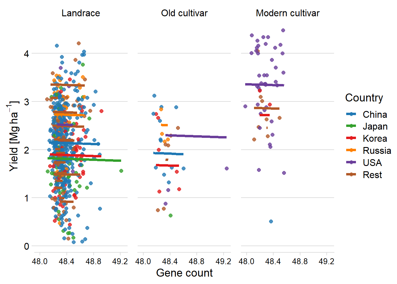

Continents, not countries

yield_country_nbs_joined_groups$continent <- countrycode(sourcevar = yield_country_nbs_joined_groups$Country,
                                                         origin = 'country.name',
                                                         destination = 'continent')

yield_country_nbs_joined_groups <- yield_country_nbs_joined_groups %>% mutate(continent2 = case_when (
  Country == 'USA' ~ 'North America',
  Country == 'Canada' ~ 'North America',
  continent == 'Americas' ~ 'South America',
  TRUE ~ continent
  ))

clm <- lm(Yield ~ Count + Group + continent2, data=yield_country_nbs_joined_groups)
summary(clm)


Call:
lm(formula = Yield ~ Count + Group + continent2, data = yield_country_nbs_joined_groups)

Residuals:
     Min       1Q   Median       3Q      Max 
-2.12554 -0.49587  0.03499  0.53143  2.18832 

Coefficients:
                         Estimate Std. Error t value Pr(>|t|)    
(Intercept)              9.547898   2.537519   3.763 0.000182 ***
Count                   -0.016487   0.005661  -2.912 0.003699 ** 
GroupOld cultivar       -0.301864   0.138459  -2.180 0.029568 *  
GroupModern cultivar     0.755298   0.198140   3.812 0.000150 ***
continent2Asia          -0.173531   0.339521  -0.511 0.609434    
continent2Europe         0.351414   0.348463   1.008 0.313566    
continent2North America  0.288662   0.371010   0.778 0.436799    
continent2Oceania       -0.738182   0.823939  -0.896 0.370595    
continent2South America -0.504629   0.476841  -1.058 0.290285    
---
Signif. codes:  0 '***' 0.001 '**' 0.01 '*' 0.05 '.' 0.1 ' ' 1

Residual standard error: 0.7511 on 722 degrees of freedom
  (10 observations deleted due to missingness)
Multiple R-squared:  0.1878,    Adjusted R-squared:  0.1788 
F-statistic: 20.87 on 8 and 722 DF,  p-value: < 2.2e-16

yield_country_nbs_joined_groups_nonacont <- yield_country_nbs_joined_groups %>% filter(!is.na(continent2))
newdat <- cbind(yield_country_nbs_joined_groups_nonacont, pred = predict(clm))

newdat %>% 
  ggplot(aes(x = Count, y = pred, color = continent2)) +
  facet_wrap( ~ Group, nrow = 1) +  
  geom_point(aes(y = Yield, color = continent2),
    alpha = 0.8,
    size = 2) +
  geom_line(aes(y=pred, group=interaction(Group, continent2),colour=continent2), size=1.5)+
  theme_minimal_hgrid() +
  xlab('Gene count') +
  ylab(expression(paste('Yield [Mg ', ha ^ -1, ']'))) +
  scale_color_manual(values = mycol) +
  #xlim(c(47.900, 49.700)) +
  labs(color = "Continent") +
  theme(panel.spacing = unit(0.9, "lines"),
  axis.text.x = element_text(size = 10))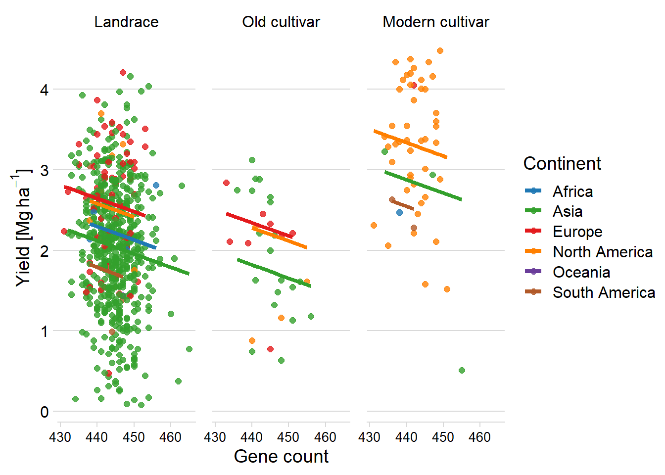

Finally, a regression by continent

I remove Oceania as there are very little individuals in there.

by_continent_model <- function(df) {
  lm(Yield ~ Count + Group, data = df)
}

with_models <- yield_country_nbs_joined_groups_nonacont %>% 
  filter(!continent2 %in% c('Africa', 'South America', 'Oceania')) %>% 
  group_by(continent2) %>% 
  nest() %>%
  mutate(models = map(data, by_continent_model))

with_models %>% mutate(glance = map(models, broom::glance)) %>% 
  unnest(glance)

# A tibble: 3 x 15
# Groups:   continent2 [3]
  continent2  data  models r.squared adj.r.squared sigma statistic p.value    df
  <chr>       <lis> <list>     <dbl>         <dbl> <dbl>     <dbl>   <dbl> <dbl>
1 Asia        <tib~ <lm>      0.0193        0.0142 0.754      3.80 1.02e-2     3
2 North Amer~ <tib~ <lm>      0.318         0.279  0.773      8.08 1.63e-4     3
3 Europe      <tib~ <lm>      0.107         0.0710 0.693      2.99 3.64e-2     3
# ... with 6 more variables: logLik <dbl>, AIC <dbl>, BIC <dbl>,
#   deviance <dbl>, df.residual <int>, nobs <int>

Let’s pull out the data

with_models %>% filter(continent2 == 'Asia') %>% unnest(data)

# A tibble: 585 x 12
# Groups:   continent2 [1]
   continent2 names presences.x `PI-ID`   Group    presences.y Yield Yield2[,1]
   <chr>      <chr>       <dbl> <chr>     <fct>          <dbl> <dbl>      <dbl>
 1 Asia       AB-01         445 PI458020  Landrace         445  1.54    -0.774 
 2 Asia       AB-02         454 PI603713  Landrace         454  1.3     -1.06  
 3 Asia       HN005         440 PI404166  Landrace         440  2.15    -0.0366
 4 Asia       HN006         448 PI407788A Landrace         448  2.06    -0.145 
 5 Asia       HN007         442 PI424298  Landrace         442  1.64    -0.653 
 6 Asia       HN008         439 PI437655  Landrace         439  2.51     0.399 
 7 Asia       HN009         445 PI495017C Landrace         445  1.85    -0.399 
 8 Asia       HN010         447 PI468915  Landrace         447  2.8      0.749 
 9 Asia       HN011         441 PI507354  Landrace         441  1.49    -0.835 
10 Asia       HN012         443 PI567305  Landrace         443  1.86    -0.387 
# ... with 575 more rows, and 4 more variables: Country <chr>, Count <dbl>,
#   continent <chr>, models <list>

plots <- with_models %>% 
  mutate(plots = map2(data, continent2, 
                      ~ ggplot(data =.x, aes(x=presences.x, y=Yield)) + 
                        geom_point() +
                        geom_smooth(method = "lm")
                      )
         )

I have no idea how to use standard facet_wrap with this.

print(plots$plots)

[[1]]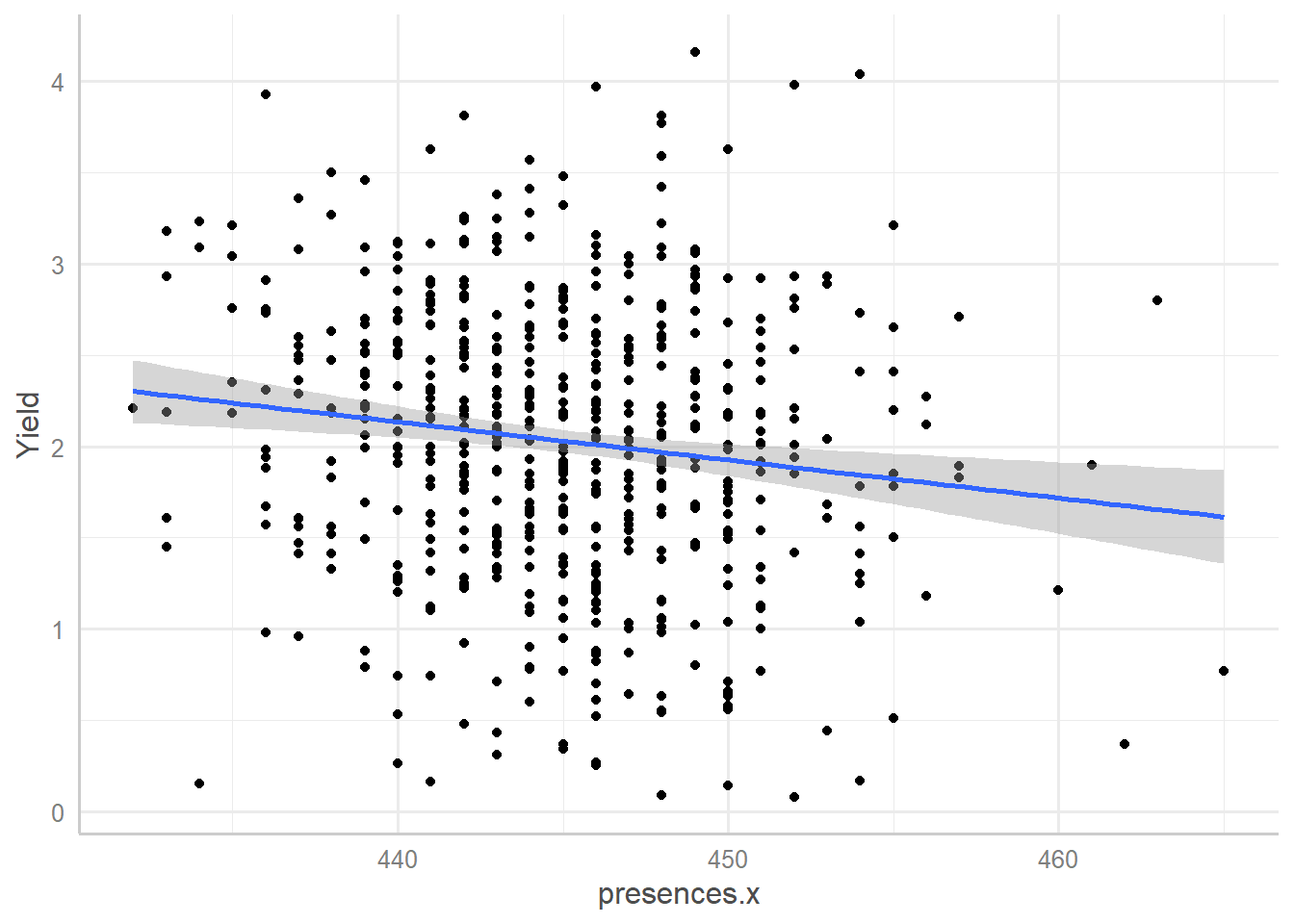


[[2]]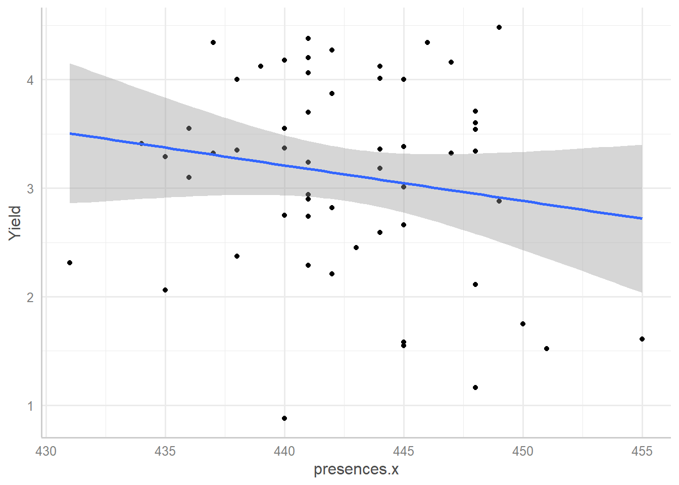


[[3]]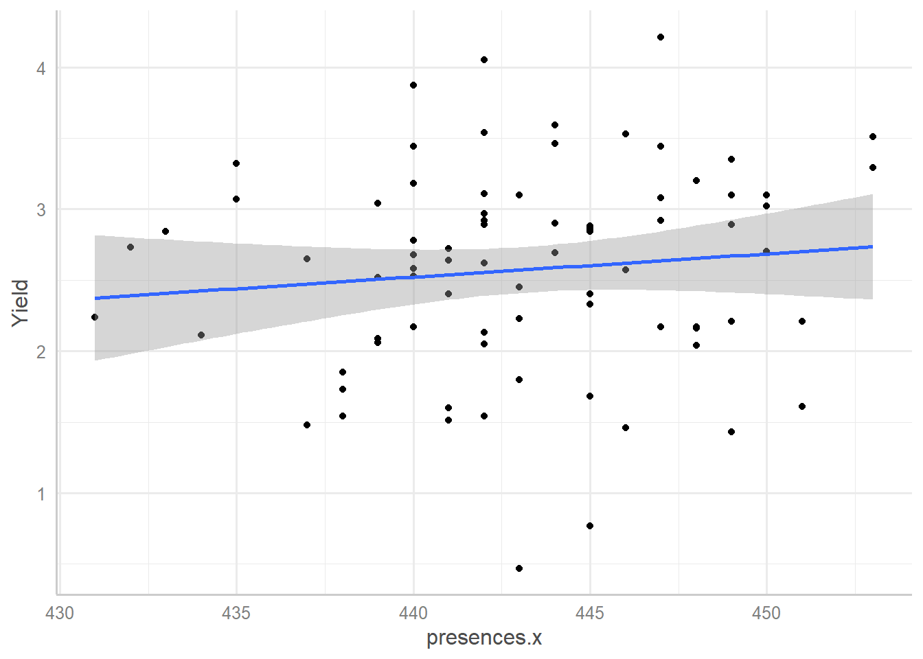

plots %>% unnest(data) %>% group_by(continent2) %>% 
  do(augment(.$models[[1]]))

# A tibble: 720 x 10
# Groups:   continent2 [3]
   continent2 Yield Count Group    .fitted  .resid    .hat .sigma     .cooksd
   <chr>      <dbl> <dbl> <fct>      <dbl>   <dbl>   <dbl>  <dbl>       <dbl>
 1 Asia        1.54   445 Landrace    2.03 -0.493  0.00178  0.754 0.000191   
 2 Asia        1.3    454 Landrace    1.85 -0.545  0.00752  0.754 0.000999   
 3 Asia        2.15   440 Landrace    2.14  0.0131 0.00348  0.754 0.000000263
 4 Asia        2.06   448 Landrace    1.97  0.0898 0.00244  0.754 0.00000868 
 5 Asia        1.64   442 Landrace    2.10 -0.455  0.00238  0.754 0.000218   
 6 Asia        2.51   439 Landrace    2.16  0.352  0.00424  0.754 0.000233   
 7 Asia        1.85   445 Landrace    2.03 -0.183  0.00178  0.754 0.0000262  
 8 Asia        2.8    447 Landrace    1.99  0.809  0.00208  0.754 0.000601   
 9 Asia        1.49   441 Landrace    2.12 -0.626  0.00286  0.754 0.000496   
10 Asia        1.86   443 Landrace    2.07 -0.214  0.00204  0.754 0.0000414  
# ... with 710 more rows, and 1 more variable: .std.resid <dbl>

Merge three figures

Let’s make Fig 1 abc instead of Fig 1,2,3

load('output/NLR_boxplot_saved.Rds') # now we have nlr_plot
merged <- (nlr_plot + fig2) / (fig1)+ plot_annotation(tag_levels='A')
cowplot::save_plot(merged, filename ='output/merged_fig1.png', base_height=3.71*2)

sessionInfo()

R version 4.1.0 (2021-05-18)
Platform: x86_64-w64-mingw32/x64 (64-bit)
Running under: Windows 10 x64 (build 19042)

Matrix products: default

locale:
[1] LC_COLLATE=English_Australia.1252  LC_CTYPE=English_Australia.1252   
[3] LC_MONETARY=English_Australia.1252 LC_NUMERIC=C                      
[5] LC_TIME=English_Australia.1252    

attached base packages:
[1] stats     graphics  grDevices utils     datasets  methods   base     

other attached packages:
 [1] broom_0.7.9        countrycode_1.3.0  RColorBrewer_1.1-2 pals_1.7          
 [5] dotwhisker_0.7.4   lmerTest_3.1-3     lme4_1.1-27.1      Matrix_1.3-3      
 [9] ggforce_0.3.3      ggsignif_0.6.3     cowplot_1.1.1      dabestr_0.3.0     
[13] magrittr_2.0.1     ggsci_2.9          sjPlot_2.8.10      modelr_0.1.8      
[17] patchwork_1.1.1    forcats_0.5.1      stringr_1.4.0      dplyr_1.0.7       
[21] purrr_0.3.4        readr_2.1.2        tidyr_1.1.4        tibble_3.1.5      
[25] ggplot2_3.3.5      tidyverse_1.3.1    workflowr_1.6.2   

loaded via a namespace (and not attached):
 [1] minqa_1.2.4         colorspace_2.0-2    ellipsis_0.3.2     
 [4] sjlabelled_1.1.8    rprojroot_2.0.2     estimability_1.3   
 [7] ggstance_0.3.5      parameters_0.15.0   fs_1.5.0           
[10] dichromat_2.0-0     rstudioapi_0.13     farver_2.1.0       
[13] bit64_4.0.5         fansi_0.5.0         mvtnorm_1.1-3      
[16] lubridate_1.8.0     xml2_1.3.2          splines_4.1.0      
[19] knitr_1.36          sjmisc_2.8.9        polyclip_1.10-0    
[22] jsonlite_1.7.2      nloptr_1.2.2.3      ggeffects_1.1.1    
[25] dbplyr_2.1.1        effectsize_0.5      mapproj_1.2.7      
[28] compiler_4.1.0      httr_1.4.2          sjstats_0.18.1     
[31] emmeans_1.7.1-1     backports_1.2.1     assertthat_0.2.1   
[34] fastmap_1.1.0       cli_3.2.0           later_1.3.0        
[37] tweenr_1.0.2        htmltools_0.5.2     tools_4.1.0        
[40] coda_0.19-4         gtable_0.3.0        glue_1.6.2         
[43] maps_3.4.0          Rcpp_1.0.7          cellranger_1.1.0   
[46] jquerylib_0.1.4     vctrs_0.3.8         nlme_3.1-152       
[49] insight_0.14.5      xfun_0.27           rvest_1.0.2        
[52] lifecycle_1.0.1     MASS_7.3-54         scales_1.1.1       
[55] vroom_1.5.7         hms_1.1.1           promises_1.2.0.1   
[58] parallel_4.1.0      yaml_2.2.1          sass_0.4.0         
[61] stringi_1.7.5       highr_0.9           bayestestR_0.11.5  
[64] boot_1.3-28         rlang_0.4.12        pkgconfig_2.0.3    
[67] evaluate_0.14       lattice_0.20-44     labeling_0.4.2     
[70] bit_4.0.4           tidyselect_1.1.1    plyr_1.8.6         
[73] R6_2.5.1            generics_0.1.1      DBI_1.1.1          
[76] mgcv_1.8-35         pillar_1.6.4        haven_2.4.3        
[79] whisker_0.4         withr_2.5.0         datawizard_0.2.1   
[82] performance_0.8.0   crayon_1.4.1        utf8_1.2.2         
[85] tzdb_0.1.2          rmarkdown_2.11      grid_4.1.0         
[88] readxl_1.3.1        git2r_0.28.0        reprex_2.0.1       
[91] digest_0.6.28       xtable_1.8-4        httpuv_1.6.3       
[94] numDeriv_2016.8-1.1 munsell_0.5.0       bslib_0.3.1

Linking yield with NLR PAV

Philipp Bayer

2020-09-22

Data loading

Linking with yield

Yield

Protein

Seed weight

Oil content

Basic lm()

Yield

Let’s nest the countries and run one lm each

FINALLY, let’s make one model per breeding group:

Protein

Seed weight

Oil content

All models together

The yield model for all genes

Continents, not countries

Finally, a regression by continent

Merge three figures