Last updated: 2022-04-01

Checks: 7 0

Knit directory: R_gene_analysis/

This reproducible R Markdown analysis was created with workflowr (version 1.6.2). The Checks tab describes the reproducibility checks that were applied when the results were created. The Past versions tab lists the development history.

R Markdown file: up-to-date

Great! Since the R Markdown file has been committed to the Git repository, you know the exact version of the code that produced these results.

Environment: empty

Great job! The global environment was empty. Objects defined in the global environment can affect the analysis in your R Markdown file in unknown ways. For reproduciblity it’s best to always run the code in an empty environment.

Seed: set.seed(20200917)

The command set.seed(20200917) was run prior to running the code in the R Markdown file. Setting a seed ensures that any results that rely on randomness, e.g. subsampling or permutations, are reproducible.

Session information: recorded

Great job! Recording the operating system, R version, and package versions is critical for reproducibility.

Cache: none

Nice! There were no cached chunks for this analysis, so you can be confident that you successfully produced the results during this run.

File paths: relative

Great job! Using relative paths to the files within your workflowr project makes it easier to run your code on other machines.

Repository version: 368c81a

Great! You are using Git for version control. Tracking code development and connecting the code version to the results is critical for reproducibility.

The results in this page were generated with repository version 368c81a. See the Past versions tab to see a history of the changes made to the R Markdown and HTML files.

Note that you need to be careful to ensure that all relevant files for the analysis have been committed to Git prior to generating the results (you can use wflow_publish or wflow_git_commit). workflowr only checks the R Markdown file, but you know if there are other scripts or data files that it depends on. Below is the status of the Git repository when the results were generated:


Ignored files:
    Ignored:    .Rhistory
    Ignored:    .Rproj.user/

Untracked files:
    Untracked:  data/Brec_R1.txt
    Untracked:  data/Brec_R2.txt
    Untracked:  data/CR15_R1.txt
    Untracked:  data/CR15_R2.txt
    Untracked:  data/CR_14_R1.txt
    Untracked:  data/CR_14_R2.txt
    Untracked:  data/KS_R1.txt
    Untracked:  data/KS_R2.txt
    Untracked:  data/NBS_PAV.txt.gz
    Untracked:  data/NLR_PAV_GD.txt
    Untracked:  data/NLR_PAV_GM.txt
    Untracked:  data/PAVs_newick.txt
    Untracked:  data/PPR1.txt
    Untracked:  data/PPR2.txt
    Untracked:  data/SNPs_lee.id.biallic_maf_0.05_geno_0.1.vcf.gz
    Untracked:  data/SNPs_newick.txt
    Untracked:  data/bac.txt
    Untracked:  data/brown.txt
    Untracked:  data/cy3.txt
    Untracked:  data/cy5.txt
    Untracked:  data/early.txt
    Untracked:  data/flowerings.txt
    Untracked:  data/foregeye.txt
    Untracked:  data/height.txt
    Untracked:  data/inds.txt
    Untracked:  data/late.txt
    Untracked:  data/mature.txt
    Untracked:  data/motting.txt
    Untracked:  data/mvp.kin.bin
    Untracked:  data/mvp.kin.desc
    Untracked:  data/oil.txt
    Untracked:  data/paperinds.txt
    Untracked:  data/pdh.txt
    Untracked:  data/protein.txt
    Untracked:  data/rust_tan.txt
    Untracked:  data/salt.txt
    Untracked:  data/seedq.txt
    Untracked:  data/seedweight.txt
    Untracked:  data/snp.gds
    Untracked:  data/stem_termination.txt
    Untracked:  data/sudden.txt
    Untracked:  data/virus.txt

Note that any generated files, e.g. HTML, png, CSS, etc., are not included in this status report because it is ok for generated content to have uncommitted changes.

These are the previous versions of the repository in which changes were made to the R Markdown (analysis/gwas.Rmd) and HTML (docs/gwas.html) files. If you’ve configured a remote Git repository (see ?wflow_git_remote), click on the hyperlinks in the table below to view the files as they were in that past version.

File	Version	Author	Date	Message
Rmd	368c81a	Philipp Bayer	2022-04-01	New analysis
html	41cccae	Philipp Bayer	2022-03-30	Build site.
Rmd	768d0c9	Philipp Bayer	2022-03-30	update GWAS with Manhattan plots
html	33c71ae	Philipp Bayer	2021-03-31	Build site.
Rmd	e6b537a	Philipp Bayer	2021-03-31	wflow_publish(“analysis/gwas.Rmd”)
html	34cbc3e	Philipp Bayer	2021-03-31	Build site.
Rmd	6f42f60	Philipp Bayer	2021-03-31	wflow_publish(“analysis/gwas.Rmd”)
html	e294dc6	Philipp Bayer	2021-03-31	Build site.
Rmd	6a6bd44	Philipp Bayer	2021-03-31	wflow_publish(“analysis/gwas.Rmd”)
html	e739391	Philipp Bayer	2021-03-31	Build site.
Rmd	dd3ab21	Philipp Bayer	2021-03-31	wflow_publish(“analysis/gwas.Rmd”)
html	bffb5ca	Philipp Bayer	2021-03-31	Build site.
Rmd	989263f	Philipp Bayer	2021-03-31	wflow_publish(“analysis/gwas.Rmd”)
html	0a3fa56	Philipp Bayer	2021-03-31	Build site.
Rmd	6bd1532	Philipp Bayer	2021-03-31	wflow_publish(“analysis/gwas.Rmd”)
html	0f3717a	Philipp Bayer	2021-03-31	Build site.
Rmd	53bc5e5	Philipp Bayer	2021-03-31	wflow_publish(“analysis/gwas.Rmd”)
html	046f90d	Philipp Bayer	2021-03-31	Build site.
Rmd	c2ccdb9	Philipp Bayer	2021-03-31	wflow_publish(“analysis/gwas.Rmd”)
html	e103452	Philipp Bayer	2021-03-31	Build site.
Rmd	8c196dc	Philipp Bayer	2021-03-31	wflow_publish(“analysis/gwas.Rmd”)
html	cf8b8b7	Philipp Bayer	2021-03-30	Build site.
Rmd	de49b61	Philipp Bayer	2021-03-30	wflow_publish(“analysis/gwas.Rmd”)
html	14c7314	Philipp Bayer	2021-03-30	Build site.
Rmd	bc094e2	Philipp Bayer	2021-03-30	wflow_publish(files = c(“analysis/gwas.Rmd”))
html	d88c271	Philipp Bayer	2021-03-30	Build site.
Rmd	c36de75	Philipp Bayer	2021-03-30	wflow_publish(c(“analysis/gwas.Rmd”))
html	51edc1f	Philipp Bayer	2021-03-30	Build site.
Rmd	e1faf81	Philipp Bayer	2021-03-30	wflow_publish(c(“analysis/gwas.Rmd”, “analysis/index.Rmd”))
html	c769673	Philipp Bayer	2021-03-29	Build site.
Rmd	764ad7b	Philipp Bayer	2021-03-29	wflow_publish(“analysis/gwas.Rmd”)
Rmd	bd5506f	Philipp Bayer	2021-03-29	missing commits
html	2844fd3	Philipp Bayer	2021-02-09	Add changes, add missing yield
html	e519122	Philipp Bayer	2020-12-11	Build site.
html	83dc49a	Philipp Bayer	2020-12-11	Trace deleted files
Rmd	dae157b	Philipp Bayer	2020-09-24	Update of analysis
html	dae157b	Philipp Bayer	2020-09-24	Update of analysis

Let’s run a GWAS via GAPIT using the NLR genes as input, and the PCs calculated using SNPs

library(GAPIT3)
library(SNPRelate)
library(ggtext)
library(tidyverse)
library(ggsignif)
library(cowplot)
library(ggsci)
library(patchwork)
library(broom)
library(ggpubr)
library(kableExtra)

Running GAPIT

First, we have to make the principal components - making them based on NLR genes alone is probably garbage. Let’s make them based on all publicly available SNPs from here.

I ran the following on a bigger server which is why it’s marked as not to run when I rerun workflowr.

if (!file.exists('data/SNPs_lee.id.biallic_maf_0.05_geno_0.1.vcf.gz')) {
  download.file('https://research-repository.uwa.edu.au/files/89232545/SNPs_lee.id.biallic_maf_0.05_geno_0.1.vcf.gz', 'data/SNPs_lee.id.biallic_maf_0.05_geno_0.1.vcf.gz')
}

#We have to convert the big vcf file

if (!file.exists("data/snp.gds")) {
  vcf.fn <- 'data/SNPs_lee.id.biallic_maf_0.05_geno_0.1.vcf.gz'
  snpgdsVCF2GDS(vcf.fn, "data/snp.gds", method="biallelic.only")
}

genofile <- snpgdsOpen('data/snp.gds')

# Let's prune the SNPs based on 0.2 LD

snpset <- snpgdsLDpruning(genofile, ld.threshold=0.2, autosome.only=F)
snpset.id <- unlist(unname(snpset))

# And now let's run the PCA
pca <- snpgdsPCA(genofile, snp.id=snpset.id, num.thread=2, autosome.only=F)

saveRDS(pca, 'data/pca.rds')

OK let’s load the results I made on the remote server and saved in a file:

# load PCA
pca <- readRDS('data/pca.rds')

A quick diagnostic plot

tab <- data.frame(sample.id = pca$sample.id,
    EV1 = pca$eigenvect[,1],    # the first eigenvector
    EV2 = pca$eigenvect[,2],    # the second eigenvector
    stringsAsFactors = FALSE)
plot(tab$EV2, tab$EV1, xlab="eigenvector 2", ylab="eigenvector 1")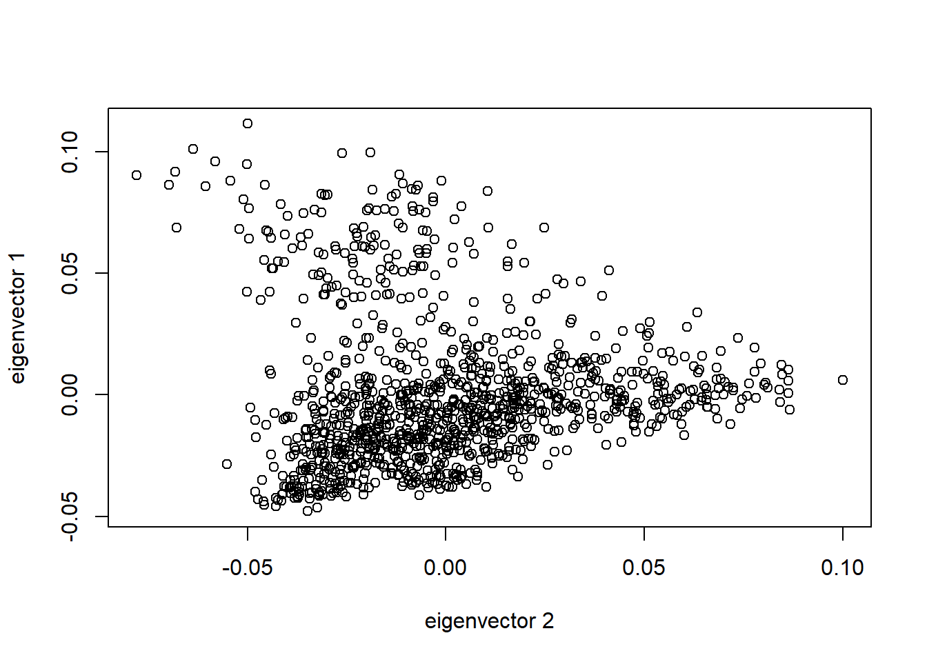

head(tab)

  sample.id           EV1         EV2
1     AB-01 -0.0096910924  0.01605862
2     AB-02  0.0061795109  0.01644249
3     BR-01 -0.0173940264 -0.01621850
4     BR-02 -0.0134548060 -0.01678429
5     BR-03 -0.0025329218 -0.03735107
6     BR-04 -0.0003749604 -0.03575687

Alright, now we have SNP-based principal components. We’ll use the first two as our own covariates in GAPIT.

I wrote a Python script which takes the NLR-only PAV table and turns that into HapMap format with fake SNPs, see code/transformToGAPIT.py.

myY <- read.table('data/yield.txt', head = TRUE)
myGD <- read.table('data/NLR_PAV_GD.txt', head = TRUE)
myGM <- read.table('data/NLR_PAV_GM.txt', head = TRUE)

GAPIT prints a LOT of stuff so I turn that off here, what’s important are all the output files.

myGAPIT <- GAPIT(
  Y=myY[,c(1,2)],
  CV = tab,
  GD = myGD,
  GM = myGM,
  PCA.total = 0, # turn off PCA calculation as I use my own based on SNPs
  model = c('GLM', 'MLM', 'MLMM', 'FarmCPU')
)

if (! dir.exists('output/GAPIT')){
  dir.create('output/GAPIT')
}

Analysing GAPIT output

R doesn’t have an in-built function to move files, so I copy and delete the output files here. There’s a package which adds file-moving but I’m not adding a whole dependency just for one convenience function, I’m not a Node.js person ;)

for(file in list.files('.', pattern='GAPIT*')) {
  file.copy(file, 'output/GAPIT')
  file.remove(file)
}

Let’s make a table of the statistically significantly associated SNPs.

results_files <- list.files('output/GAPIT/', pattern='*GWAS.Results.csv', full.names = T)

Let’s use FDR < 0.05 as cutoff

results_df <- NULL
for(i in seq_along(results_files)) {
  this_df <- read_csv(results_files[i])
  filt_df <- this_df %>% filter(`FDR_Adjusted_P-values` < 0.05)
  
  # pull the method name out and add to dataframe
  this_method <- str_split(results_files[i], "\\.")[[1]][2]
  filt_df <- filt_df %>% add_column(Method = this_method, .before = 'SNP')
  if (is.null(results_df)) {
    results_df <- filt_df
  } else {
    results_df <- rbind(results_df, filt_df)
  }
}

Rows: 486 Columns: 10

-- Column specification --------------------------------------------------------
Delimiter: ","
chr (1): SNP
dbl (7): Chromosome, Position, P.value, maf, nobs, FDR_Adjusted_P-values, ef...
lgl (2): Rsquare.of.Model.without.SNP, Rsquare.of.Model.with.SNP


i Use `spec()` to retrieve the full column specification for this data.
i Specify the column types or set `show_col_types = FALSE` to quiet this message.

Rows: 486 Columns: 10

-- Column specification --------------------------------------------------------
Delimiter: ","
chr (1): SNP
dbl (9): Chromosome, Position, P.value, maf, nobs, Rsquare.of.Model.without....


i Use `spec()` to retrieve the full column specification for this data.
i Specify the column types or set `show_col_types = FALSE` to quiet this message.

Rows: 486 Columns: 10

-- Column specification --------------------------------------------------------
Delimiter: ","
chr (1): SNP
dbl (9): Chromosome, Position, P.value, maf, nobs, Rsquare.of.Model.without....


i Use `spec()` to retrieve the full column specification for this data.
i Specify the column types or set `show_col_types = FALSE` to quiet this message.

Rows: 486 Columns: 10

-- Column specification --------------------------------------------------------
Delimiter: ","
chr (1): SNP
dbl (6): Chromosome, Position, P.value, maf, nobs, FDR_Adjusted_P-values
lgl (3): Rsquare.of.Model.without.SNP, Rsquare.of.Model.with.SNP, effect


i Use `spec()` to retrieve the full column specification for this data.
i Specify the column types or set `show_col_types = FALSE` to quiet this message.

results_df %>% kbl() %>%  kable_styling()

Method	SNP	Chromosome	Position	P.value	maf	nobs	Rsquare.of.Model.without.SNP	Rsquare.of.Model.with.SNP	FDR_Adjusted_P-values	effect
FarmCPU	GlymaLee.02G228600.1.p	2	49198872	0.0000038	0.0013004	769	NA	NA	0.0018691	-1.7185122
FarmCPU	UWASoyPan04354	22	277	0.0000373	0.1040312	769	NA	NA	0.0090673	0.1505357
FarmCPU	UWASoyPan00316	22	405	0.0000813	0.1235371	769	NA	NA	0.0131697	-0.1361126
FarmCPU	GlymaLee.01G030900.1.p	1	3567950	0.0001897	0.4928479	769	NA	NA	0.0230510	0.0837741
FarmCPU	UWASoyPan00772	22	326	0.0002724	0.1976593	769	NA	NA	0.0264748	0.1073770
FarmCPU	GlymaLee.14G022000.1.p	14	1789365	0.0004215	0.2236671	769	NA	NA	0.0341436	-0.0953602
GLM	GlymaLee.02G228600.1.p	2	49198872	0.0000000	0.0013004	769	0.3795503	0.4064602	0.0000058	-1.9354957
GLM	UWASoyPan04354	22	277	0.0000150	0.1040312	769	0.3795503	0.3949224	0.0036512	0.1706430
GLM	UWASoyPan00772	22	326	0.0000315	0.1976593	769	0.3795503	0.3937506	0.0051105	0.1291152
GLM	UWASoyPan00316	22	405	0.0000446	0.1235371	769	0.3795503	0.3932066	0.0054160	-0.1498671
GLM	GlymaLee.16G111300.1.p	16	30996392	0.0001209	0.0676203	769	0.3795503	0.3916447	0.0117547	0.1830838
GLM	UWASoyPan00022	22	958	0.0003783	0.0364109	769	0.3795503	0.3898773	0.0267416	0.2285028
GLM	GlymaLee.01G030900.1.p	1	3567950	0.0003852	0.4928479	769	0.3795503	0.3898498	0.0267416	0.0861666
MLM	GlymaLee.02G228600.1.p	2	49198872	0.0000005	0.0013004	769	0.4220320	0.4413330	0.0002584	-1.6924714
MLMM	GlymaLee.02G228600.1.p	2	49198872	0.0000003	0.0013004	769	NA	NA	0.0001373	NA

Ah beautiful, one NLR gene found by all methods, and a bunch of extra pangenome genes found by FarmCPU/GLM. However the one gene found by all methods has a horrible MAF so we’ll probably end up ignoring that.

results_df %>% group_by(SNP) %>% count() %>% arrange(n)

# A tibble: 8 x 2
# Groups:   SNP [8]
  SNP                        n
  <chr>                  <int>
1 GlymaLee.14G022000.1.p     1
2 GlymaLee.16G111300.1.p     1
3 UWASoyPan00022             1
4 GlymaLee.01G030900.1.p     2
5 UWASoyPan00316             2
6 UWASoyPan00772             2
7 UWASoyPan04354             2
8 GlymaLee.02G228600.1.p     4

candidates <- results_df %>% 
  group_by(SNP) %>% 
  count() %>% 
  filter(n >= 2)

candidates %>% knitr::kable()

SNP	n
GlymaLee.01G030900.1.p	2
GlymaLee.02G228600.1.p	4
UWASoyPan00316	2
UWASoyPan00772	2
UWASoyPan04354	2

Let’s focus on genes found by more than one method.

This particular R-gene GlymaLee.02G228600.1.p seems to have a strong negative impact on yield (effect -1.69 in MLM, -1.94 in GLM, -1.72 in FarmCPU) but it also has a horrible MAF, normally this would get filtered in SNPs but we don’t have SNPs here. Let’s plot the yield for individuals who have vs those who don’t have those genes that appear in more than one method.

pav_table <- read_tsv('./data/soybean_pan_pav.matrix_gene.txt.gz')

Rows: 51414 Columns: 1111

-- Column specification --------------------------------------------------------
Delimiter: "\t"
chr    (1): Individual
dbl (1110): AB-01, AB-02, BR-01, BR-02, BR-03, BR-04, BR-05, BR-06, BR-07, B...


i Use `spec()` to retrieve the full column specification for this data.
i Specify the column types or set `show_col_types = FALSE` to quiet this message.

yield <- read_tsv('./data/yield.txt')

Rows: 769 Columns: 2

-- Column specification --------------------------------------------------------
Delimiter: "\t"
chr (1): Line
dbl (1): Yield


i Use `spec()` to retrieve the full column specification for this data.
i Specify the column types or set `show_col_types = FALSE` to quiet this message.

pav_table %>% 
  filter(Individual == 'GlymaLee.02G228600.1.p') %>% 
  pivot_longer(!Individual, names_to = 'Line', values_to = 'Presence') %>% 
  inner_join(yield) %>% arrange(Presence) %>% head()

Joining, by = "Line"

# A tibble: 6 x 4
  Individual             Line    Presence Yield
  <chr>                  <chr>      <dbl> <dbl>
1 GlymaLee.02G228600.1.p USB-762        0  2.88
2 GlymaLee.02G228600.1.p AB-01          1  1.54
3 GlymaLee.02G228600.1.p AB-02          1  1.3 
4 GlymaLee.02G228600.1.p For            1  3.34
5 GlymaLee.02G228600.1.p HN001          1  3.54
6 GlymaLee.02G228600.1.p HN005          1  2.15

OK this gene is ‘boring’ - it’s lost only in a single line, and we can’t trust that. We’ll remove it.

pav_table %>% 
  filter(Individual == 'GlymaLee.02G228600.1.p') %>% 
  pivot_longer(!Individual, names_to = 'Line', values_to = 'Presence') %>% 
  inner_join(yield) %>% 
  summarise(median_y= median(Yield))

Joining, by = "Line"

# A tibble: 1 x 1
  median_y
     <dbl>
1     2.18

At least this particular line with the lost gene has slightly higher yield than the median? but soooo many different reasons… Let’s remove this gene as MAF < 5%.

Let’s check the other genes.

candidates <- candidates %>% 
  filter(SNP != 'GlymaLee.02G228600.1.p')
candidates %>% knitr::kable()

SNP	n
GlymaLee.01G030900.1.p	2
UWASoyPan00316	2
UWASoyPan00772	2
UWASoyPan04354	2

Visualising per-gene differences

plots <- list()
for(i in 1:nrow(candidates)) {
  this_cand = candidates[i,]
  p <- pav_table %>% 
    filter(Individual == this_cand$SNP) %>% 
    pivot_longer(!Individual, names_to = 'Line', values_to = 'Presence') %>% 
    inner_join(yield) %>% 
    mutate(Presence = case_when(
      Presence == 0.0 ~ 'Lost',
      Presence == 1.0 ~ 'Present'
    )) %>% 
    ggplot(aes(x=Presence, y = Yield, group=Presence)) + 
    geom_boxplot() + 
    geom_jitter(alpha=0.9, size=0.4) + 
    geom_signif(comparisons = list(c('Lost', 'Present')), 
              map_signif_level = T) +
    theme_minimal_hgrid()
    #xlab(paste('Presence', str_replace(this_cand$SNP, '.1.p',''))) # make the gene name a bit nicer
  plots[[i]] <- p
}

Joining, by = "Line"
Joining, by = "Line"
Joining, by = "Line"
Joining, by = "Line"

wrap_plots(plots) + 
  plot_annotation(tag_levels = 'A')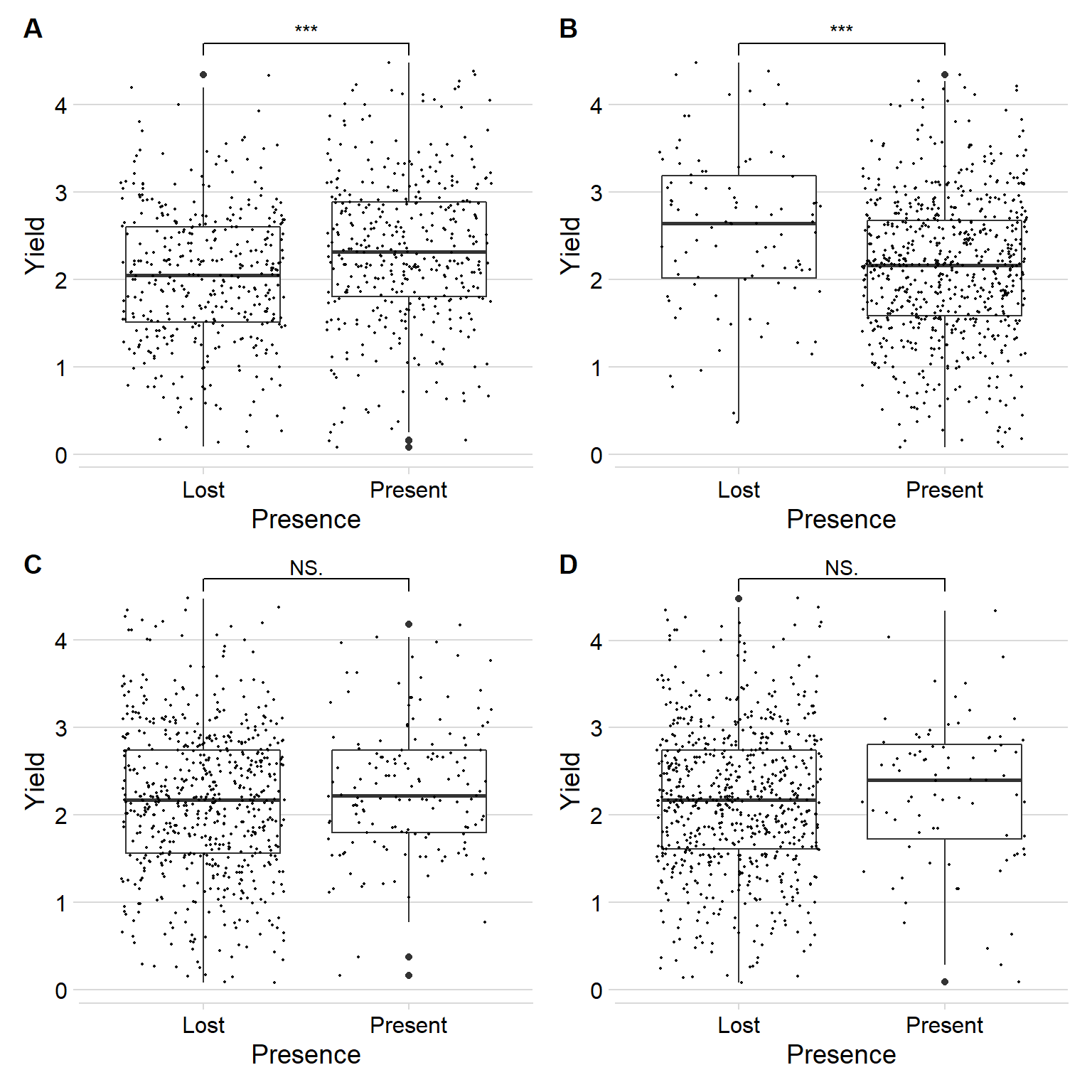

Four nice plots we have now, we’ll use those as supplementary. It’s interesting how the reference gene has a positive impact on yield, the pangenome extra gene has a negative impact, and the other two don’t do much. Then again there are many reasons why we see this outcome.

For myself, the four labels: GlymaLee.01G030900.1.p, UWASoyPan00316, UWASoyPan00772, UWASoyPan04354

Let’s also make those plots, grouped by breeding group

groups <- read_csv('./data/Table_of_cultivar_groups.csv')

Rows: 1069 Columns: 3

-- Column specification --------------------------------------------------------
Delimiter: ","
chr (3): Data-storage-ID, PI-ID, Group in violin table


i Use `spec()` to retrieve the full column specification for this data.
i Specify the column types or set `show_col_types = FALSE` to quiet this message.

groups <- groups %>% dplyr::rename(Group = `Group in violin table`)
groups <- groups %>% 
  mutate(Group = str_replace_all(Group, 'landrace', 'Landrace')) %>%
  mutate(Group = str_replace_all(Group, 'Old_cultivar', 'Old cultivar')) %>%
  mutate(Group = str_replace_all(Group, 'Modern_cultivar', 'Modern cultivar')) %>%
  mutate(Group = str_replace_all(Group, 'Wild-type', 'Wild'))

groups$Group <-
  factor(
    groups$Group,
    levels = c('Wild',
               'Landrace',
               'Old cultivar',
               'Modern cultivar')
  )

npg_col = pal_npg("nrc")(9)

col_list <- c(`Wild`=npg_col[8],
   Landrace = npg_col[3],
  `Old cultivar`=npg_col[2],
  `Modern cultivar`=npg_col[4])


plots <- list()
for(i in 1:nrow(candidates)) {
  this_cand = candidates[i,]
  p <- pav_table %>% 
    filter(Individual == this_cand$SNP) %>% 
    pivot_longer(!Individual, names_to = 'Line', values_to = 'Presence') %>% 
    inner_join(yield) %>% 
    inner_join(groups, by = c('Line'='Data-storage-ID')) %>% 
    mutate(Presence = case_when(
      Presence == 0.0 ~ 'Lost',
      Presence == 1.0 ~ 'Present'
    )) %>% 
    ggplot(aes(x=Presence, y = Yield, group=Presence, color=Group)) + 
    geom_boxplot() + 
    geom_jitter(alpha=0.9, size=0.4) + 
    facet_wrap(~Group) +
    geom_signif(comparisons = list(c('Lost', 'Present')), 
              map_signif_level = T) +
    theme_minimal_hgrid() +
    ylab(expression(paste('Yield [Mg ', ha ^ -1, ']'))) +
    scale_color_manual(values = col_list)

  plots[[i]] <- p
}

Joining, by = "Line"
Joining, by = "Line"
Joining, by = "Line"
Joining, by = "Line"

wrap_plots(plots) + 
  plot_annotation(tag_levels = 'A') +
  plot_layout(guides='collect') & theme(legend.position = 'none')

Warning in wilcox.test.default(c(2.19, 2.6, 2.74, 1.63, 1.61, 2.45, 1.21, :
cannot compute exact p-value with ties

Warning in wilcox.test.default(c(4, 2.66, 1.52, 2.47, 4.34, 2.21, 3.23, : cannot
compute exact p-value with ties

Warning in wilcox.test.default(c(2.66, 1.54, 2.21, 0.77, 2.84, 2.51, 0.89:
cannot compute exact p-value with ties

Warning in wilcox.test.default(c(4.38, 4.16, 4, 4.48, 4.12, 3.24, 2.59, : cannot
compute exact p-value with ties

Warning in wilcox.test.default(c(2.19, 2.6, 2.74, 1.63, 2.88, 2.29, 2.17, :
cannot compute exact p-value with ties

Warning in wilcox.test.default(c(3.54, 4.38, 4.16, 4.05, 4.06, 2.75, 4.27, :
cannot compute exact p-value with ties

Warning in wilcox.test.default(c(2.19, 2.66, 2.6, 2.74, 1.63, 1.61, 1.21, :
cannot compute exact p-value with ties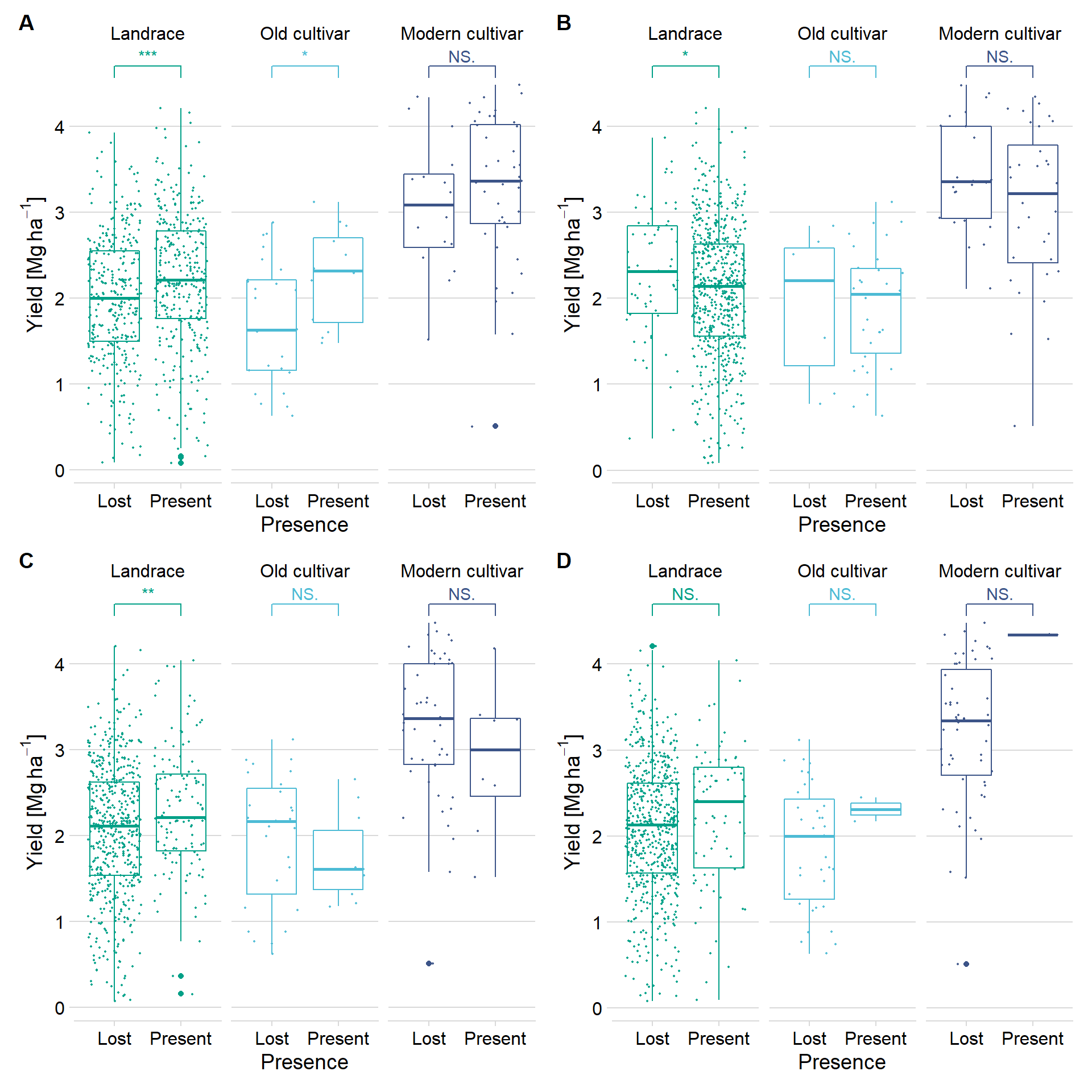

I also need a presence/absence percentage for all candidates

big_t <- NULL
for(i in 1:nrow(candidates)) {
  this_cand = candidates[i,]
  t <- pav_table %>% 
    filter(Individual == this_cand$SNP) %>% 
    pivot_longer(!Individual, names_to = 'Line', values_to = 'Presence') %>%
    inner_join(groups, by = c('Line'='Data-storage-ID')) %>% group_by(Group) %>% 
    dplyr::select(Presence, Group) %>% 
    table() %>% as_tibble()
  #t <- t %>% add_column(Presence=c(0,1), .before = '.')
  t<- t %>% add_column(Gene=this_cand$SNP, .before='Presence')
  if(is.null(big_t)) {
    big_t <- t
  } else {
    big_t <- rbind(big_t, t)
  }
}

big_t %>% group_by(Group, Gene) %>% mutate(group_sum = sum(n)) %>% 
  mutate(`Percentage` = n/group_sum*100) %>% 
  dplyr::select(-group_sum) %>% 
  rename(Count=n) %>% 
  mutate(Presence = case_when(
      Presence == 0.0 ~ 'Lost',
      Presence == 1.0 ~ 'Present'
    ))  %>%
  knitr::kable(digits=2)

Gene	Presence	Group	Count	Percentage
GlymaLee.01G030900.1.p	Lost	Wild	29	18.47
GlymaLee.01G030900.1.p	Present	Wild	128	81.53
GlymaLee.01G030900.1.p	Lost	Landrace	359	49.65
GlymaLee.01G030900.1.p	Present	Landrace	364	50.35
GlymaLee.01G030900.1.p	Lost	Old cultivar	30	65.22
GlymaLee.01G030900.1.p	Present	Old cultivar	16	34.78
GlymaLee.01G030900.1.p	Lost	Modern cultivar	41	28.67
GlymaLee.01G030900.1.p	Present	Modern cultivar	102	71.33
UWASoyPan00316	Lost	Wild	14	8.92
UWASoyPan00316	Present	Wild	143	91.08
UWASoyPan00316	Lost	Landrace	68	9.41
UWASoyPan00316	Present	Landrace	655	90.59
UWASoyPan00316	Lost	Old cultivar	9	19.57
UWASoyPan00316	Present	Old cultivar	37	80.43
UWASoyPan00316	Lost	Modern cultivar	71	49.65
UWASoyPan00316	Present	Modern cultivar	72	50.35
UWASoyPan00772	Lost	Wild	71	45.22
UWASoyPan00772	Present	Wild	86	54.78
UWASoyPan00772	Lost	Landrace	586	81.05
UWASoyPan00772	Present	Landrace	137	18.95
UWASoyPan00772	Lost	Old cultivar	32	69.57
UWASoyPan00772	Present	Old cultivar	14	30.43
UWASoyPan00772	Lost	Modern cultivar	126	88.11
UWASoyPan00772	Present	Modern cultivar	17	11.89
UWASoyPan04354	Lost	Wild	87	55.41
UWASoyPan04354	Present	Wild	70	44.59
UWASoyPan04354	Lost	Landrace	636	87.97
UWASoyPan04354	Present	Landrace	87	12.03
UWASoyPan04354	Lost	Old cultivar	44	95.65
UWASoyPan04354	Present	Old cultivar	2	4.35
UWASoyPan04354	Lost	Modern cultivar	141	98.60
UWASoyPan04354	Present	Modern cultivar	2	1.40

big_t %>% group_by(Group, Gene) %>% mutate(group_sum = sum(n)) %>%
  mutate(Gene = str_replace_all(Gene, '.1.p','')) %>% 
  mutate(`Percentage` = n/group_sum*100) %>% 
  dplyr::select(-group_sum) %>% 
  filter(Presence == '1') %>% 
  mutate(Group = factor(Group, levels=c('Wild', 'Landrace', 'Old cultivar', 'Modern cultivar'))) %>% 
  ggplot(aes(x = Group, y = Percentage, group=Gene, color=Gene)) + 
  geom_line(size=1.5) +
  theme_minimal_hgrid() +
  ylab('Percentage present') +
  scale_color_brewer(palette = 'Dark2') +
  theme(axis.text.x = element_text(angle = -45, hjust=0))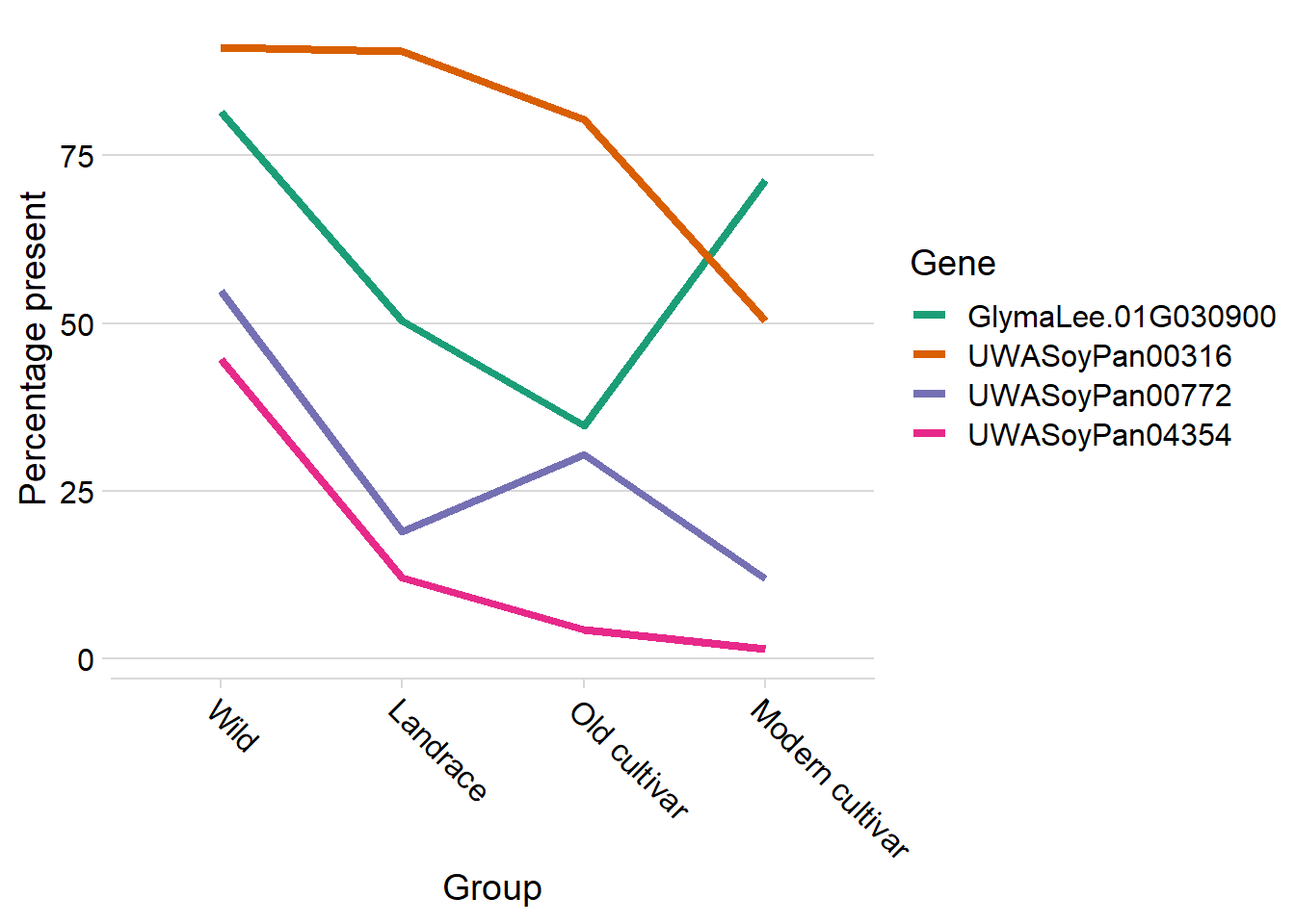

and let’s also get the per-gene mean and median yield

yields <- NULL
for(i in 1:nrow(candidates)) {
  this_cand = candidates[i,]
  this_t <- pav_table %>% 
    filter(Individual == this_cand$SNP) %>% 
    pivot_longer(!Individual, names_to = 'Line', values_to = 'Presence') %>% 
    inner_join(yield) %>%
    inner_join(groups, by = c('Line'='Data-storage-ID')) %>% 
    group_by(Presence, Group) %>% 
    summarise(`Mean yield` = mean(Yield)) %>% 
    add_column(Gene=this_cand$SNP, .before='Presence') %>% 
    arrange(Group)
  if (is.null(yields)) {
    yields <- this_t
  } else {
    yields <- rbind(yields, this_t)
  }
}

Joining, by = "Line"

`summarise()` has grouped output by 'Presence'. You can override using the `.groups` argument.

Joining, by = "Line"

`summarise()` has grouped output by 'Presence'. You can override using the `.groups` argument.

Joining, by = "Line"

`summarise()` has grouped output by 'Presence'. You can override using the `.groups` argument.

Joining, by = "Line"

`summarise()` has grouped output by 'Presence'. You can override using the `.groups` argument.

yields %>% knitr::kable(digits=2)

Gene	Presence	Group	Mean yield
GlymaLee.01G030900.1.p	0	Landrace	2.00
GlymaLee.01G030900.1.p	1	Landrace	2.22
GlymaLee.01G030900.1.p	0	Old cultivar	1.73
GlymaLee.01G030900.1.p	1	Old cultivar	2.27
GlymaLee.01G030900.1.p	0	Modern cultivar	3.06
GlymaLee.01G030900.1.p	1	Modern cultivar	3.28
UWASoyPan00316	0	Landrace	2.29
UWASoyPan00316	1	Landrace	2.09
UWASoyPan00316	0	Old cultivar	1.92
UWASoyPan00316	1	Old cultivar	1.90
UWASoyPan00316	0	Modern cultivar	3.42
UWASoyPan00316	1	Modern cultivar	3.06
UWASoyPan00772	0	Landrace	2.06
UWASoyPan00772	1	Landrace	2.30
UWASoyPan00772	0	Old cultivar	1.97
UWASoyPan00772	1	Old cultivar	1.74
UWASoyPan00772	0	Modern cultivar	3.27
UWASoyPan00772	1	Modern cultivar	2.89
UWASoyPan04354	0	Landrace	2.09
UWASoyPan04354	1	Landrace	2.24
UWASoyPan04354	0	Old cultivar	1.88
UWASoyPan04354	1	Old cultivar	2.31
UWASoyPan04354	0	Modern cultivar	3.20
UWASoyPan04354	1	Modern cultivar	4.34

yields %>% 
  group_by(Gene, Group) %>% 
  summarise('Yield difference when gene present' = diff(`Mean yield`)) %>% 
  knitr::kable(digits=2)

`summarise()` has grouped output by 'Gene'. You can override using the `.groups` argument.

Gene	Group	Yield difference when gene present
GlymaLee.01G030900.1.p	Landrace	0.21
GlymaLee.01G030900.1.p	Old cultivar	0.54
GlymaLee.01G030900.1.p	Modern cultivar	0.22
UWASoyPan00316	Landrace	-0.20
UWASoyPan00316	Old cultivar	-0.01
UWASoyPan00316	Modern cultivar	-0.36
UWASoyPan00772	Landrace	0.24
UWASoyPan00772	Old cultivar	-0.23
UWASoyPan00772	Modern cultivar	-0.39
UWASoyPan04354	Landrace	0.15
UWASoyPan04354	Old cultivar	0.43
UWASoyPan04354	Modern cultivar	1.14

Better kinship modeling

A reviewer pointed out that this post-hoc analysis does not account for kinship, so let’s make it a bit nicer by using PC1 and PC2 as covariates.

big_t <- list()
for(i in 1:nrow(candidates)) {
  this_cand = candidates[i,]
  p <- pav_table %>% 
    filter(Individual == this_cand$SNP) %>% 
    pivot_longer(!Individual, names_to = 'Line', values_to = 'Presence') %>% 
    inner_join(yield) %>% 
    inner_join(groups, by = c('Line'='Data-storage-ID')) %>% 
    mutate(Presence = case_when(
      Presence == 0.0 ~ 'Lost',
      Presence == 1.0 ~ 'Present'
    ))
  # now get EV1/EV2 (PC1,PC2)
  p <- p %>% left_join(tab, by=c('Line'='sample.id'))
  big_t[[this_cand$SNP]] <- tidy(lm(Yield ~ Presence + Group + EV1 + EV2, data=p)) %>% 
    filter(term == 'PresencePresent')
}

Joining, by = "Line"
Joining, by = "Line"
Joining, by = "Line"
Joining, by = "Line"

big_t <- bind_rows(big_t, .id='gene')
big_t %>% kbl() %>%  kable_styling()

gene	term	estimate	std.error	statistic	p.value
GlymaLee.01G030900.1.p	PresencePresent	0.1555618	0.0533526	2.915731	0.0036537
UWASoyPan00316	PresencePresent	-0.2801745	0.0827615	-3.385325	0.0007477
UWASoyPan00772	PresencePresent	0.1374274	0.0670730	2.048924	0.0408147
UWASoyPan04354	PresencePresent	0.2813016	0.0853339	3.296480	0.0010248

All p < 0.05, just like the GWAS. Estimates are all positive except for one gene. Let’s also correct for multiple testing

big_t$FDR <- p.adjust(big_t$p.value)
big_t %>% kbl() %>%  kable_styling()

gene	term	estimate	std.error	statistic	p.value	FDR
GlymaLee.01G030900.1.p	PresencePresent	0.1555618	0.0533526	2.915731	0.0036537	0.0073073
UWASoyPan00316	PresencePresent	-0.2801745	0.0827615	-3.385325	0.0007477	0.0029908
UWASoyPan00772	PresencePresent	0.1374274	0.0670730	2.048924	0.0408147	0.0408147
UWASoyPan04354	PresencePresent	0.2813016	0.0853339	3.296480	0.0010248	0.0030745

Same as before. Now let’s run this for every single group.

bigger_t <- list()
for(i in 1:nrow(candidates)) {
  this_cand = candidates[i,]
  p <- pav_table %>% 
    filter(Individual == this_cand$SNP) %>% 
    pivot_longer(!Individual, names_to = 'Line', values_to = 'Presence') %>% 
    inner_join(yield) %>% 
    inner_join(groups, by = c('Line'='Data-storage-ID')) %>% 
    mutate(Presence = case_when(
      Presence == 0.0 ~ 'Lost',
      Presence == 1.0 ~ 'Present'
    ))
  p <- p %>% left_join(tab, by=c('Line'='sample.id'))
  # now iterate over the groups
  for( x in unique(p$Group)) {
    subp <- p %>% filter(Group == x)
    
    print(i)
    print(x)
    thisname <- paste(this_cand$SNP, x, sep='')
    bigger_t[[thisname]] <- tidy(lm(Yield ~ Presence + EV1 + EV2, data=subp)) %>% 
      filter(term == 'PresencePresent')
  }  
}

Joining, by = "Line"

[1] 1
[1] "Landrace"
[1] 1
[1] "Modern cultivar"
[1] 1
[1] "Old cultivar"

Joining, by = "Line"

[1] 2
[1] "Landrace"
[1] 2
[1] "Modern cultivar"
[1] 2
[1] "Old cultivar"

Joining, by = "Line"

[1] 3
[1] "Landrace"
[1] 3
[1] "Modern cultivar"
[1] 3
[1] "Old cultivar"

Joining, by = "Line"

[1] 4
[1] "Landrace"
[1] 4
[1] "Modern cultivar"
[1] 4
[1] "Old cultivar"

bigger_t <- bind_rows(bigger_t, .id='gene')
bigger_t$FDR <- p.adjust(bigger_t$p.value)
bigger_t %>% kbl() %>%  kable_styling()

gene	term	estimate	std.error	statistic	p.value	FDR
GlymaLee.01G030900.1.pLandrace	PresencePresent	0.1411758	0.0558536	2.5276054	0.0117152	0.1054369
GlymaLee.01G030900.1.pModern cultivar	PresencePresent	0.2364309	0.2425475	0.9747819	0.3341815	1.0000000
GlymaLee.01G030900.1.pOld cultivar	PresencePresent	0.5199299	0.2641657	1.9681958	0.0574943	0.4599541
UWASoyPan00316Landrace	PresencePresent	-0.2983311	0.0949330	-3.1425447	0.0017494	0.0209928
UWASoyPan00316Modern cultivar	PresencePresent	-0.3305952	0.2230181	-1.4823688	0.1442775	0.8656653
UWASoyPan00316Old cultivar	PresencePresent	0.1437413	0.3224778	0.4457403	0.6586956	1.0000000
UWASoyPan00772Landrace	PresencePresent	0.1879880	0.0708854	2.6519981	0.0081928	0.0819276
UWASoyPan00772Modern cultivar	PresencePresent	-0.3719740	0.3139092	-1.1849736	0.2414154	1.0000000
UWASoyPan00772Old cultivar	PresencePresent	-0.2529017	0.2643518	-0.9566861	0.3456823	1.0000000
UWASoyPan04354Landrace	PresencePresent	0.2581922	0.0863727	2.9892807	0.0028997	0.0318966
UWASoyPan04354Modern cultivar	PresencePresent	1.3645257	0.7918797	1.7231476	0.0908042	0.6356295
UWASoyPan04354Old cultivar	PresencePresent	0.5391899	0.5247666	1.0274851	0.3116649	1.0000000

bigger_t %>% filter(FDR < 0.05) %>% kbl() %>%  kable_styling()

gene	term	estimate	std.error	statistic	p.value	FDR
UWASoyPan00316Landrace	PresencePresent	-0.2983311	0.0949330	-3.142545	0.0017494	0.0209928
UWASoyPan04354Landrace	PresencePresent	0.2581922	0.0863727	2.989281	0.0028997	0.0318966

OK let’s remake the above plots only with these two p-values

my_test <- function(x = NULL, y = NULL) {
  print(y)
  results <- tidy(lm(Yield ~ Presence + Group + EV1 + EV2))
  return(results)
}
plots <- list()
for(i in 1:nrow(candidates)) {
  this_cand = candidates[i,]
  p <- pav_table %>% 
    filter(Individual == this_cand$SNP) %>% 
    pivot_longer(!Individual, names_to = 'Line', values_to = 'Presence') %>% 
    inner_join(yield) %>% 
    inner_join(groups, by = c('Line'='Data-storage-ID')) %>% 
    mutate(Presence = case_when(
      Presence == 0.0 ~ 'Lost',
      Presence == 1.0 ~ 'Present'
    )) %>% 
    left_join(tab, by=c('Line'='sample.id')) %>% 
    ggplot(aes(x=Presence, 
               y = Yield, 
               group=Presence, 
               color=Group)) + 
    geom_boxplot() + 
    geom_jitter(alpha=0.9, size=0.4) + 
    facet_wrap(~Group) +
    geom_signif(comparisons = list(c('Lost', 'Present')), 
              test = 'my_test',
              map_signif_level = T) +
    theme_minimal_hgrid() +
    ylab(expression(paste('Yield [Mg ', ha ^ -1, ']'))) +
    scale_color_manual(values = col_list)

  plots[[i]] <- p
}

Joining, by = "Line"
Joining, by = "Line"
Joining, by = "Line"
Joining, by = "Line"

# 
# wrap_plots(plots) + 
#   plot_annotation(tag_levels = 'A') +
#   plot_layout(guides='collect') & theme(legend.position = 'none')

Manhattan plots

A reviewer asked for Manhattan plots.

# slightly modified from https://danielroelfs.com/blog/how-i-create-manhattan-plots-using-ggplot/
# Thanks :) 
myplot <- function(f) {
  print(f)
  mlm <- read_csv(paste('./output/GAPIT/', f, sep=''))
  mlm <- mlm %>% filter(SNP != 'GlymaLee.02G228600.1.p')
  data_cum <- mlm %>% 
    group_by(Chromosome) %>% 
    summarise(max_bp = max(Position)) %>% 
    mutate(bp_add = lag(cumsum(max_bp), default = 0)) %>% 
    select(Chromosome, bp_add)
  
  mlm <- mlm %>% 
    inner_join(data_cum, by = "Chromosome") %>% 
    mutate(bp_cum = Position + bp_add)
  
  axis_set <- mlm %>% 
    group_by(Chromosome) %>% 
    summarize(center = mean(bp_cum))
  
  ylim <- mlm %>% 
     filter(`FDR_Adjusted_P-values` == min(`FDR_Adjusted_P-values`)) %>% 
     mutate(ylim = abs(floor(log10(`FDR_Adjusted_P-values`))) + 1) %>% 
     pull(ylim)
  
  mlm_plot <- ggplot(mlm, aes(x = bp_cum, y = -log10(`FDR_Adjusted_P-values`), 
                color = as_factor(Chromosome))) +
    geom_hline(yintercept = -log10(0.05), color = "grey40", linetype = "dashed") + 
    geom_point(alpha = 0.75) +
    scale_x_continuous(label = axis_set$Chromosome, breaks = axis_set$center) +
    scale_y_continuous(expand = c(0,0), limits = c(0, ylim)) +
    scale_color_manual(values = rep(c("#276FBF", "#183059"), unique(length(axis_set$Chromosome)))) +
    labs(x = NULL, 
         y = "-log<sub>10</sub>(p)") + 
    theme_minimal() +
    theme( 
      legend.position = "none",
      panel.border = element_blank(),
      panel.grid.major.x = element_blank(),
      panel.grid.minor.x = element_blank(),
      axis.title.y = element_markdown(),
      #axis.text.x = element_text(angle = 60, size = 8, vjust = 0.5)
    )
mlm_plot
}

files <- list.files(path='./output/GAPIT/', '*GWAS.Results.csv')
names(files) <- str_split(files, pattern = '\\.', simplify=T)[,2]
# remove MLM as there are no hits
files <- files[c('GLM','MLMM','FarmCPU')]
plot_list <- lapply(files, myplot)

[1] "GAPIT.GLM.Yield.GWAS.Results.csv"

Rows: 486 Columns: 10

-- Column specification --------------------------------------------------------
Delimiter: ","
chr (1): SNP
dbl (9): Chromosome, Position, P.value, maf, nobs, Rsquare.of.Model.without....


i Use `spec()` to retrieve the full column specification for this data.
i Specify the column types or set `show_col_types = FALSE` to quiet this message.

[1] "GAPIT.MLMM.Yield.GWAS.Results.csv"

Rows: 486 Columns: 10

-- Column specification --------------------------------------------------------
Delimiter: ","
chr (1): SNP
dbl (6): Chromosome, Position, P.value, maf, nobs, FDR_Adjusted_P-values
lgl (3): Rsquare.of.Model.without.SNP, Rsquare.of.Model.with.SNP, effect


i Use `spec()` to retrieve the full column specification for this data.
i Specify the column types or set `show_col_types = FALSE` to quiet this message.

[1] "GAPIT.FarmCPU.Yield.GWAS.Results.csv"

Rows: 486 Columns: 10

-- Column specification --------------------------------------------------------
Delimiter: ","
chr (1): SNP
dbl (7): Chromosome, Position, P.value, maf, nobs, FDR_Adjusted_P-values, ef...
lgl (2): Rsquare.of.Model.without.SNP, Rsquare.of.Model.with.SNP


i Use `spec()` to retrieve the full column specification for this data.
i Specify the column types or set `show_col_types = FALSE` to quiet this message.

result <- plot_list$GLM /  plot_list$FarmCPU + plot_annotation(tag_levels = 'A')

result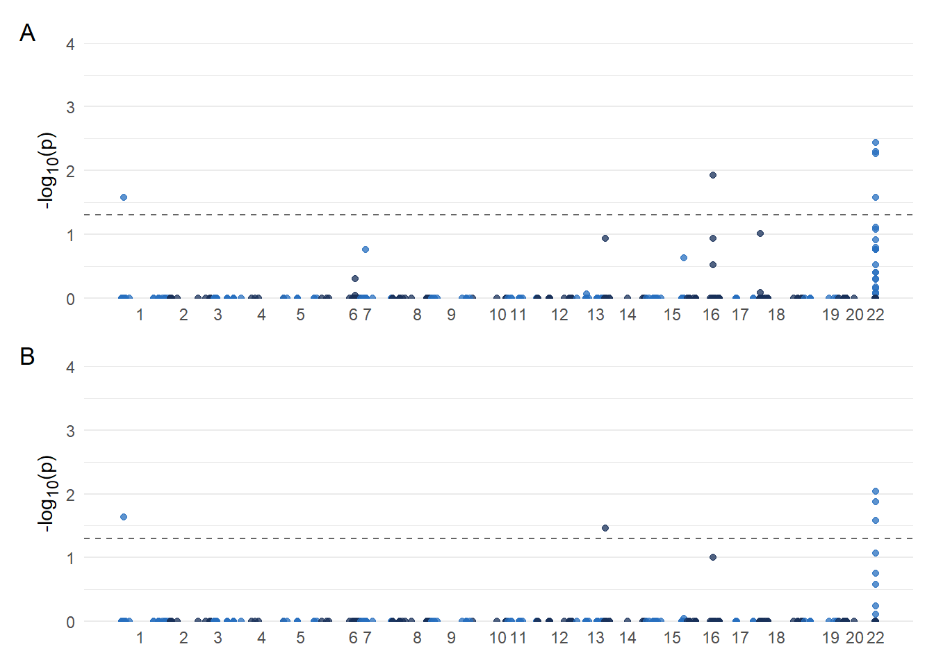

cowplot::save_plot(filename = 'output/GWAS_Manhattan.png',result, base_height = 5, base_width=8)

sessionInfo()

R version 4.1.0 (2021-05-18)
Platform: x86_64-w64-mingw32/x64 (64-bit)
Running under: Windows 10 x64 (build 19042)

Matrix products: default

locale:
[1] LC_COLLATE=English_Australia.1252  LC_CTYPE=English_Australia.1252   
[3] LC_MONETARY=English_Australia.1252 LC_NUMERIC=C                      
[5] LC_TIME=English_Australia.1252    

attached base packages:
[1] stats     graphics  grDevices utils     datasets  methods   base     

other attached packages:
 [1] kableExtra_1.3.4 ggpubr_0.4.0     broom_0.7.9      patchwork_1.1.1 
 [5] ggsci_2.9        cowplot_1.1.1    ggsignif_0.6.3   forcats_0.5.1   
 [9] stringr_1.4.0    dplyr_1.0.7      purrr_0.3.4      readr_2.1.2     
[13] tidyr_1.1.4      tibble_3.1.5     ggplot2_3.3.5    tidyverse_1.3.1 
[17] ggtext_0.1.1     SNPRelate_1.26.0 gdsfmt_1.28.1    GAPIT3_3.1.0    
[21] workflowr_1.6.2 

loaded via a namespace (and not attached):
 [1] fs_1.5.0           bit64_4.0.5        lubridate_1.8.0    RColorBrewer_1.1-2
 [5] webshot_0.5.2      httr_1.4.2         rprojroot_2.0.2    tools_4.1.0       
 [9] backports_1.2.1    bslib_0.3.1        utf8_1.2.2         R6_2.5.1          
[13] DBI_1.1.1          colorspace_2.0-2   withr_2.5.0        tidyselect_1.1.1  
[17] bit_4.0.4          compiler_4.1.0     git2r_0.28.0       cli_3.2.0         
[21] rvest_1.0.2        xml2_1.3.2         labeling_0.4.2     sass_0.4.0        
[25] scales_1.1.1       systemfonts_1.0.4  digest_0.6.28      rmarkdown_2.11    
[29] svglite_2.1.0      pkgconfig_2.0.3    htmltools_0.5.2    dbplyr_2.1.1      
[33] fastmap_1.1.0      highr_0.9          rlang_0.4.12       readxl_1.3.1      
[37] rstudioapi_0.13    farver_2.1.0       jquerylib_0.1.4    generics_0.1.1    
[41] jsonlite_1.7.2     vroom_1.5.7        car_3.0-12         magrittr_2.0.1    
[45] Rcpp_1.0.7         munsell_0.5.0      fansi_0.5.0        abind_1.4-5       
[49] lifecycle_1.0.1    stringi_1.7.5      whisker_0.4        yaml_2.2.1        
[53] carData_3.0-5      grid_4.1.0         parallel_4.1.0     promises_1.2.0.1  
[57] crayon_1.4.1       haven_2.4.3        gridtext_0.1.4     hms_1.1.1         
[61] knitr_1.36         pillar_1.6.4       markdown_1.1       reprex_2.0.1      
[65] glue_1.6.2         evaluate_0.14      modelr_0.1.8       vctrs_0.3.8       
[69] tzdb_0.1.2         httpuv_1.6.3       cellranger_1.1.0   gtable_0.3.0      
[73] assertthat_0.2.1   xfun_0.27          rstatix_0.7.0      later_1.3.0       
[77] viridisLite_0.4.0  ellipsis_0.3.2

R-gene count comparisons

Philipp Bayer

2020-09-18

Running GAPIT

Analysing GAPIT output

Visualising per-gene differences

Better kinship modeling

Manhattan plots