Last updated: 2020-12-11

Checks: 7 0

Knit directory: R_gene_analysis/

This reproducible R Markdown analysis was created with workflowr (version 1.6.2.9000). The Checks tab describes the reproducibility checks that were applied when the results were created. The Past versions tab lists the development history.

R Markdown file: up-to-date

Great! Since the R Markdown file has been committed to the Git repository, you know the exact version of the code that produced these results.

Environment: empty

Great job! The global environment was empty. Objects defined in the global environment can affect the analysis in your R Markdown file in unknown ways. For reproduciblity it’s best to always run the code in an empty environment.

Seed: set.seed(20200917)

The command set.seed(20200917) was run prior to running the code in the R Markdown file. Setting a seed ensures that any results that rely on randomness, e.g. subsampling or permutations, are reproducible.

Session information: recorded

Great job! Recording the operating system, R version, and package versions is critical for reproducibility.

Cache: none

Nice! There were no cached chunks for this analysis, so you can be confident that you successfully produced the results during this run.

File paths: relative

Great job! Using relative paths to the files within your workflowr project makes it easier to run your code on other machines.

Repository version: 83dc49a

Great! You are using Git for version control. Tracking code development and connecting the code version to the results is critical for reproducibility.

The results in this page were generated with repository version 83dc49a. See the Past versions tab to see a history of the changes made to the R Markdown and HTML files.

Note that you need to be careful to ensure that all relevant files for the analysis have been committed to Git prior to generating the results (you can use wflow_publish or wflow_git_commit). workflowr only checks the R Markdown file, but you know if there are other scripts or data files that it depends on. Below is the status of the Git repository when the results were generated:


Ignored files:
    Ignored:    .Rhistory
    Ignored:    .Rproj.user/

Untracked files:
    Untracked:  data/Brec_R1.txt
    Untracked:  data/Brec_R2.txt
    Untracked:  data/CR15_R1.txt
    Untracked:  data/CR15_R2.txt
    Untracked:  data/CR_14_R1.txt
    Untracked:  data/CR_14_R2.txt
    Untracked:  data/KS_R1.txt
    Untracked:  data/KS_R2.txt
    Untracked:  data/NBS_PAV.txt.gz
    Untracked:  data/NLR_PAV_GD.txt
    Untracked:  data/NLR_PAV_GM.txt
    Untracked:  data/PAVs_newick.txt
    Untracked:  data/PPR1.txt
    Untracked:  data/PPR2.txt
    Untracked:  data/SNPs_newick.txt
    Untracked:  data/bac.txt
    Untracked:  data/brown.txt
    Untracked:  data/cy3.txt
    Untracked:  data/cy5.txt
    Untracked:  data/early.txt
    Untracked:  data/flowerings.txt
    Untracked:  data/foregeye.txt
    Untracked:  data/height.txt
    Untracked:  data/late.txt
    Untracked:  data/mature.txt
    Untracked:  data/motting.txt
    Untracked:  data/mvp.kin.bin
    Untracked:  data/mvp.kin.desc
    Untracked:  data/oil.txt
    Untracked:  data/pdh.txt
    Untracked:  data/protein.txt
    Untracked:  data/rust_tan.txt
    Untracked:  data/salt.txt
    Untracked:  data/seedq.txt
    Untracked:  data/seedweight.txt
    Untracked:  data/stem_termination.txt
    Untracked:  data/sudden.txt
    Untracked:  data/virus.txt
    Untracked:  data/yield.txt

Note that any generated files, e.g. HTML, png, CSS, etc., are not included in this status report because it is ok for generated content to have uncommitted changes.

These are the previous versions of the repository in which changes were made to the R Markdown (analysis/first-analysis.Rmd) and HTML (docs/first-analysis.html) files. If you’ve configured a remote Git repository (see ?wflow_git_remote), click on the hyperlinks in the table below to view the files as they were in that past version.

File	Version	Author	Date	Message
html	83dc49a	Philipp Bayer	2020-12-11	Trace deleted files
html	dae157b	Philipp Bayer	2020-09-24	Update of analysis
Rmd	1b346e9	Philipp Bayer	2020-09-22	More data!
html	1b346e9	Philipp Bayer	2020-09-22	More data!
html	0777e1d	Philipp Bayer	2020-09-22	update
html	e6e9b9b	Philipp Bayer	2020-09-21	Build site.
Rmd	c1fbbf9	Philipp Bayer	2020-09-21	wflow_publish("analysis/*")
Rmd	c71005a	Philipp Bayer	2020-09-18	lots changes
html	c71005a	Philipp Bayer	2020-09-18	lots changes
html	7d33bac	Philipp Bayer	2020-09-18	Build site.
Rmd	695db1e	Philipp Bayer	2020-09-18	wflow_publish(c(“analysis/eda.Rmd”, “analysis/first-analysis.Rmd”,
html	ca65f66	Philipp Bayer	2020-09-18	Build site.
Rmd	efd6af1	Philipp Bayer	2020-09-18	wflow_git_commit(all = T)
html	efd6af1	Philipp Bayer	2020-09-18	wflow_git_commit(all = T)

knitr::opts_chunk$set(warning = FALSE, message = FALSE) 
library(tidyverse)
library(patchwork)
library(ggsci)
library(dabestr)
library(dabestr)
library(cowplot)
library(ggsignif)

theme_set(theme_cowplot())

Introduction

npg_col = pal_npg("nrc")(9)
col_list <- c(`Wild-type`=npg_col[8],
   Landrace = npg_col[3],
  `Old cultivar`=npg_col[2],
  `Modern cultivar`=npg_col[4])

pav_table <- read_tsv('./data/soybean_pan_pav.matrix_gene.txt.gz')

NBS part

Let’s pull the NBS genes from the table

nbs <- read_tsv('./data/Lee.NBS.candidates.lst', col_names = c('Name', 'Class'))
# have to remove the .t1s 
nbs$Name <- gsub('.t1','', nbs$Name)

nbs_pav_table <- pav_table %>% filter(Individual %in% nbs$Name)

names <- c()
percs <- c()

for (i in seq_along(nbs_pav_table)){
  if ( i == 1) next
  thisind <- colnames(nbs_pav_table)[i]
  pavs <- nbs_pav_table[[i]]
  perc <- sum(pavs) / length(pavs) * 100
  names <- c(names, thisind)
  percs <- c(percs, perc)
}
nbs_res_tibb <- new_tibble(list(names = names, percs = percs))

OK what do these presence percentages look like?

ggplot(data=nbs_res_tibb, aes(x=percs)) + geom_histogram(bins=25)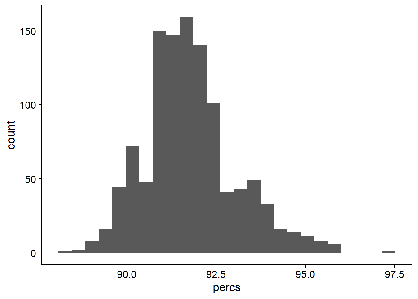

On average, 91.7701034% of NBS genes are present in each individual.

Now let’s join the table of presences to the four different types so we can group these numbers.

nbs_groups <- read_csv('./data/Table_of_cultivar_groups.csv')
nbs_joined_groups <- left_join(nbs_res_tibb, nbs_groups, by = c('names'='Data-storage-ID'))

nbs_joined_groups$`Group in violin table` <- gsub('landrace', 'Landrace', nbs_joined_groups$`Group in violin table`)
nbs_joined_groups$`Group in violin table` <- gsub('Modern_cultivar', 'Modern cultivar', nbs_joined_groups$`Group in violin table`)
nbs_joined_groups$`Group in violin table` <- gsub('Old_cultivar', 'Old cultivar', nbs_joined_groups$`Group in violin table`)

nbs_joined_groups$`Group in violin table` <- factor(nbs_joined_groups$`Group in violin table`, levels=c(NA, 'Wild-type', 'Landrace', 'Old cultivar', 'Modern cultivar'))

library(ggforce)
nbs_vio <- nbs_joined_groups %>% filter(`Group in violin table` != 'NA') %>% 
  ggplot(aes(y=percs, x=`Group in violin table`, fill=`Group in violin table`)) + 
  geom_violin(draw_quantiles = c(0.5)) +
  geom_sina(alpha=0.5) +
  geom_smooth(aes(group=1), method='glm') +
  scale_fill_manual(values=col_list)+
  guides(fill = FALSE) +
  ylim(c(87, 100))

nbs_vio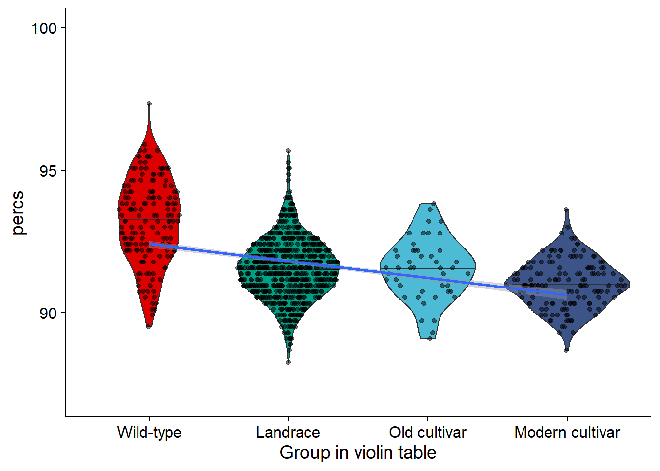

nbs_joined_groups %>% filter(`Group in violin table` != 'NA') %>% 
  ggplot(aes(y=percs, x=`Group in violin table`, fill=`Group in violin table`)) + 
  geom_smooth(aes(group=1), method='lm', se = FALSE) +
  geom_jitter() +
  scale_fill_manual(values=col_list)+
  guides(fill = FALSE)# +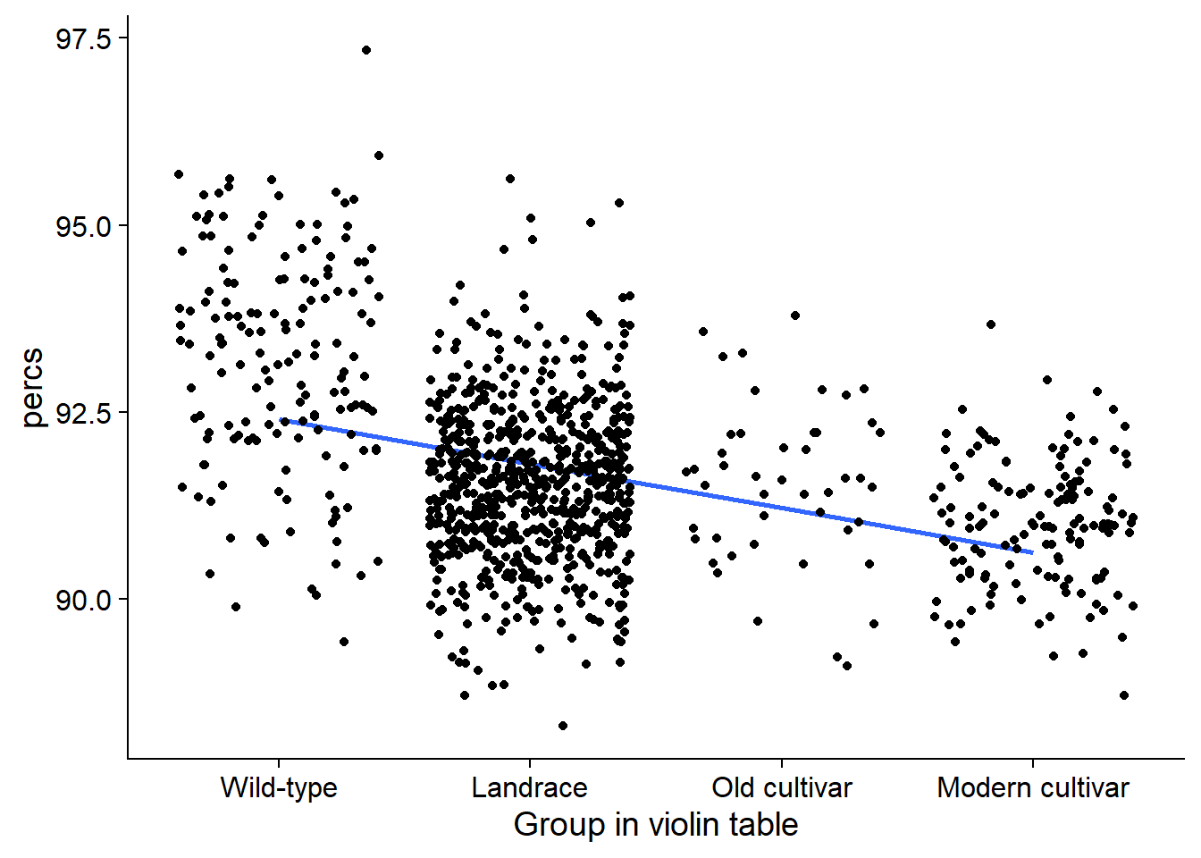

  #ylim(c(0, 100))

nbs_joined_groups %>% filter(!is.na(`PI-ID`)) %>% 
  group_by(`Group in violin table`) %>% 
  summarise(min_perc = min(percs),
            max_perc = max(percs),
            mean_perc = mean(percs),
            median_perc = median(percs),
            std_perc = sd(percs)) %>% 
  knitr::kable()

Group in violin table	min_perc	max_perc	mean_perc	median_perc	std_perc
Wild-type	89.50617	97.32510	93.19939	93.20988	1.4754746
Landrace	88.27160	95.67901	91.54130	91.56379	1.0312082
Old cultivar	89.09465	93.82716	91.53695	91.56379	1.0701423
Modern cultivar	88.68313	93.62140	91.01125	90.94650	0.8329189

RLK part

Let’s do the same plot with RLKs

rlk <- read_tsv('./data/Lee.RLK.candidates.lst', col_names = c('Name', 'Class', 'Subtype'))

# have to remove the .t1s 
rlk$Name <- gsub('.t1','', rlk$Name)

rlk_pav_table <- pav_table %>% filter(Individual %in% rlk$Name)

names <- c()
percs <- c()

for (i in seq_along(rlk_pav_table)){
  if ( i == 1) next
  thisind <- colnames(rlk_pav_table)[i]
  pavs <- rlk_pav_table[[i]]
  perc <- sum(pavs) / length(pavs) * 100
  names <- c(names, thisind)
  percs <- c(percs, perc)
}
rlk_res_tibb <- new_tibble(list(names = names, percs = percs))

OK what do these presence percentages look like?

ggplot(data=rlk_res_tibb, aes(x=percs)) + geom_histogram(bins=25)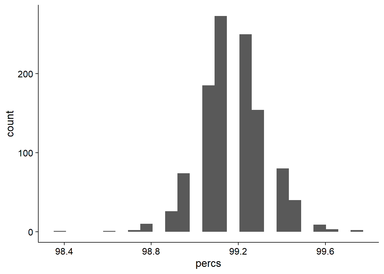

On average, 99.190418% of NBS genes are present in each individual.

Now let’s join the table of presences to the four different types so we can group these numbers.

groups <- read_csv('./data/Table_of_cultivar_groups.csv')

rlk_joined_groups <- left_join(rlk_res_tibb, groups, by = c('names'='Data-storage-ID'))

rlk_joined_groups$`Group in violin table` <- gsub('landrace', 'Landrace', rlk_joined_groups$`Group in violin table`)
rlk_joined_groups$`Group in violin table` <- gsub('Modern_cultivar', 'Modern cultivar', rlk_joined_groups$`Group in violin table`)
rlk_joined_groups$`Group in violin table` <- gsub('Old_cultivar', 'Old cultivar', rlk_joined_groups$`Group in violin table`)

rlk_joined_groups$`Group in violin table` <- factor(rlk_joined_groups$`Group in violin table`, levels=c(NA, 'Wild-type', 'Landrace', 'Old cultivar', 'Modern cultivar'))

rlk_vio <- rlk_joined_groups %>% filter(`Group in violin table` != 'NA') %>% 
  ggplot(aes(y=percs, x=`Group in violin table`, fill=`Group in violin table`)) + 
  geom_violin(draw_quantiles = c(0.5)) +
  geom_sina(alpha=0.5) +
  geom_smooth(aes(group=1), method='lm', se = FALSE) +
  scale_fill_manual(values=col_list)+
  guides(fill = FALSE)# +
  #ylim(c(87, 100))
rlk_vio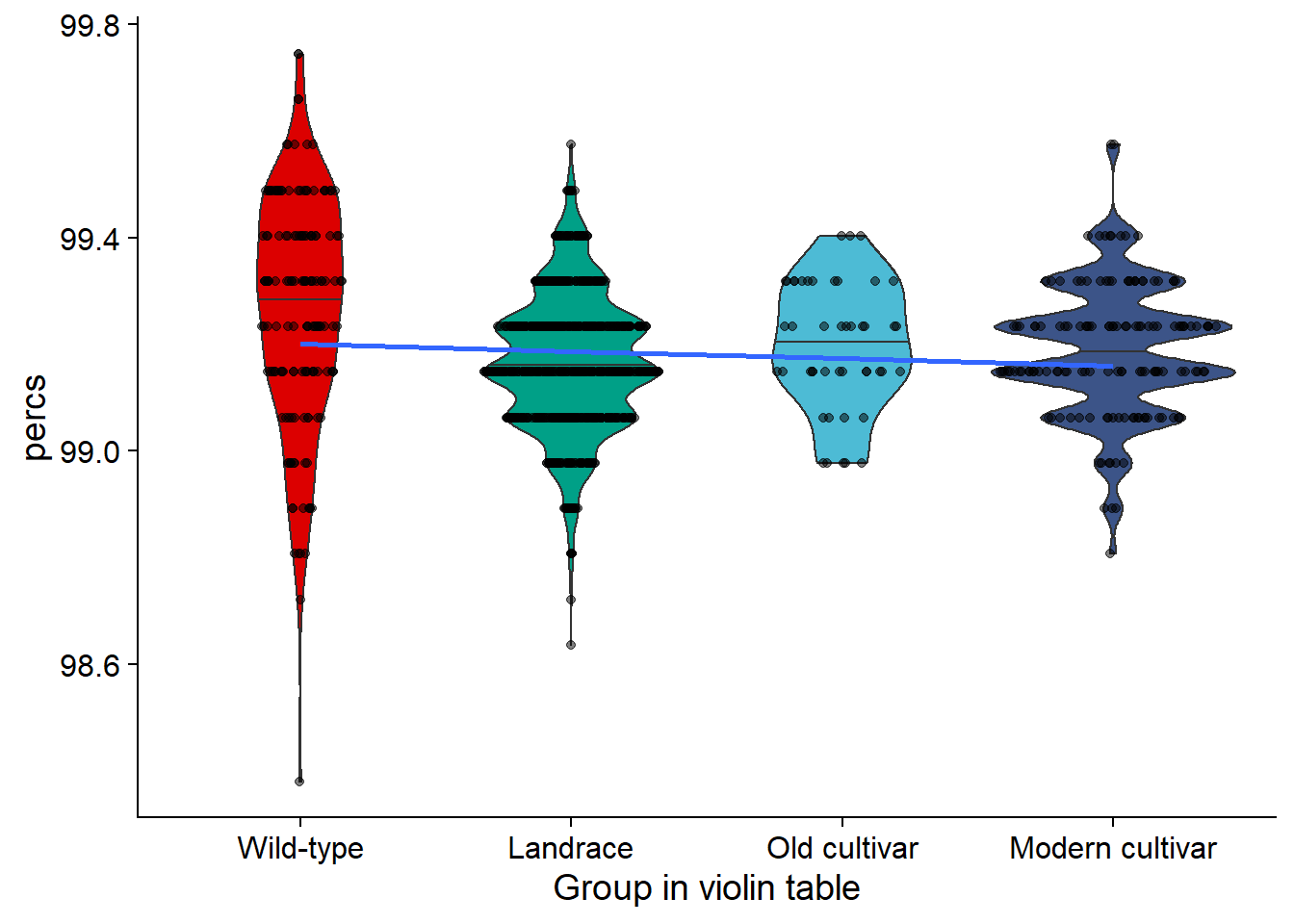

rlk_joined_groups %>% filter(!is.na(`PI-ID`)) %>% 
  group_by(`Group in violin table`) %>% 
  summarise(min_perc = min(percs),
            max_perc = max(percs),
            mean_perc = mean(percs),
            median_perc = median(percs),
            std_perc = sd(percs)) %>% 
  knitr::kable()

Group in violin table	min_perc	max_perc	mean_perc	median_perc	std_perc
Wild-type	98.38022	99.74425	99.26314	99.31799	0.2177805
Landrace	98.63598	99.57374	99.16600	99.14749	0.1278145
Old cultivar	98.97698	99.40324	99.19752	99.23274	0.1199946
Modern cultivar	98.80648	99.57374	99.18922	99.14749	0.1255006

RLP part

And now with RLPs

rlp <- read_tsv('./data/Lee.RLP.candidates.lst', col_names = c('Name', 'Class', 'Subtype'))

# have to remove the .t1s 
rlp$Name <- gsub('.t1','', rlp$Name)

rlp_pav_table <- pav_table %>% filter(Individual %in% rlp$Name)

names <- c()
percs <- c()

for (i in seq_along(rlp_pav_table)){
  if ( i == 1) next
  thisind <- colnames(rlp_pav_table)[i]
  pavs <- rlp_pav_table[[i]]
  perc <- sum(pavs) / length(pavs) * 100
  names <- c(names, thisind)
  percs <- c(percs, perc)
}
rlp_res_tibb <- new_tibble(list(names = names, percs = percs))

OK what do these presence percentages look like?

ggplot(data=rlp_res_tibb, aes(x=percs)) + geom_histogram(bins=25)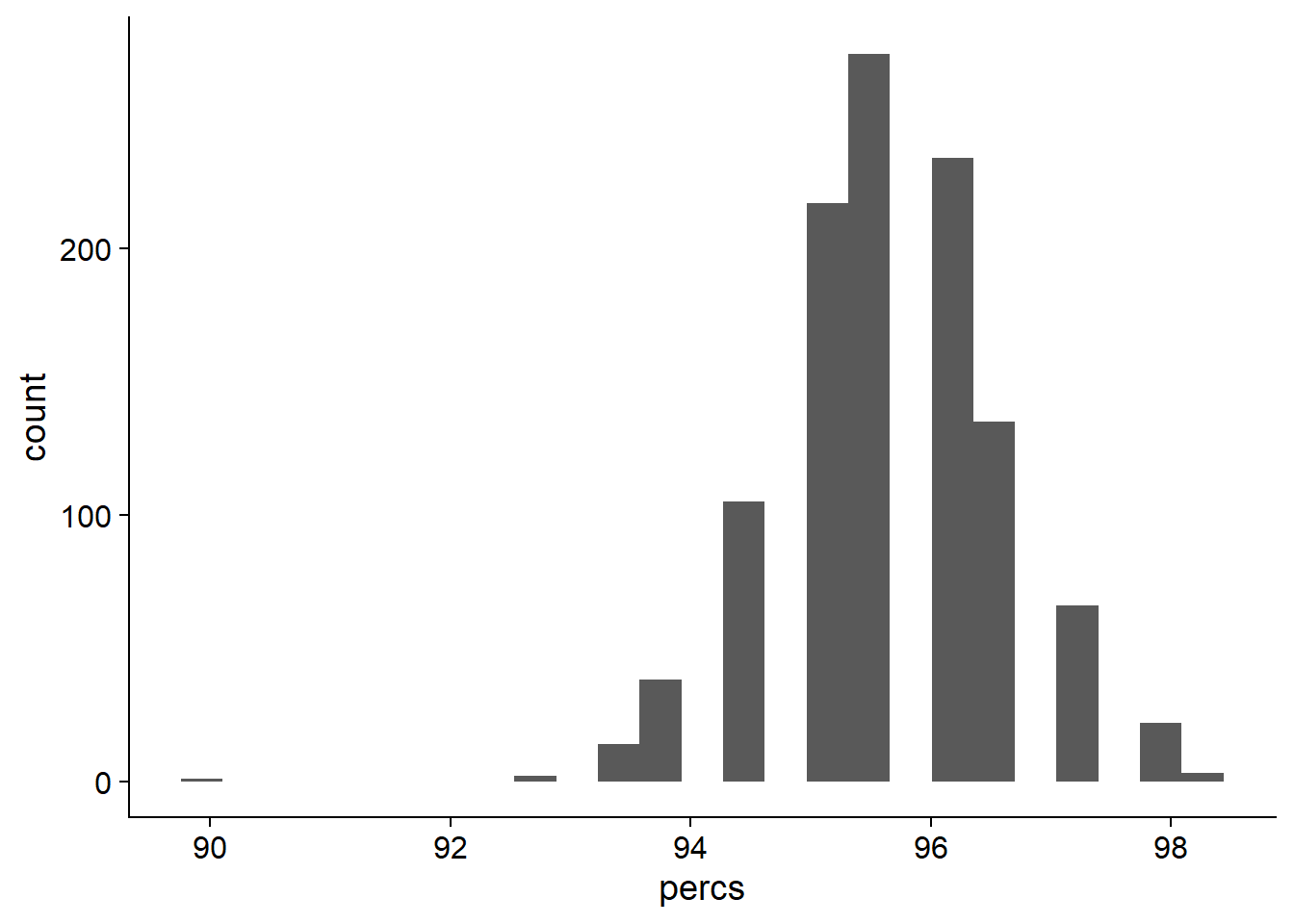

On average, 95.6496496% of NBS genes are present in each individual.

Now let’s join the table of presences to the four different types so we can group these numbers.

groups <- read_csv('./data/Table_of_cultivar_groups.csv')
rlp_joined_groups <- left_join(rlp_res_tibb, groups, by = c('names'='Data-storage-ID'))

rlp_joined_groups$`Group in violin table` <- gsub('landrace', 'Landrace', rlp_joined_groups$`Group in violin table`)
rlp_joined_groups$`Group in violin table` <- gsub('Modern_cultivar', 'Modern cultivar', rlp_joined_groups$`Group in violin table`)
rlp_joined_groups$`Group in violin table` <- gsub('Old_cultivar', 'Old cultivar', rlp_joined_groups$`Group in violin table`)

rlp_joined_groups$`Group in violin table` <- factor(rlp_joined_groups$`Group in violin table`, levels=c(NA, 'Wild-type', 'Landrace', 'Old cultivar', 'Modern cultivar'))

rlp_vio <- rlp_joined_groups %>% filter(`Group in violin table` != 'NA') %>% 
  ggplot(aes(y=percs, x=`Group in violin table`, fill=`Group in violin table`)) + 
  geom_violin(draw_quantiles = c(0.5)) +
  geom_sina(alpha=0.5) +
    geom_smooth(aes(group=1), method='lm', se = FALSE) +
  scale_fill_manual(values=col_list)+
  guides(fill = FALSE) +
  ylim(c(87, 100))
rlp_vio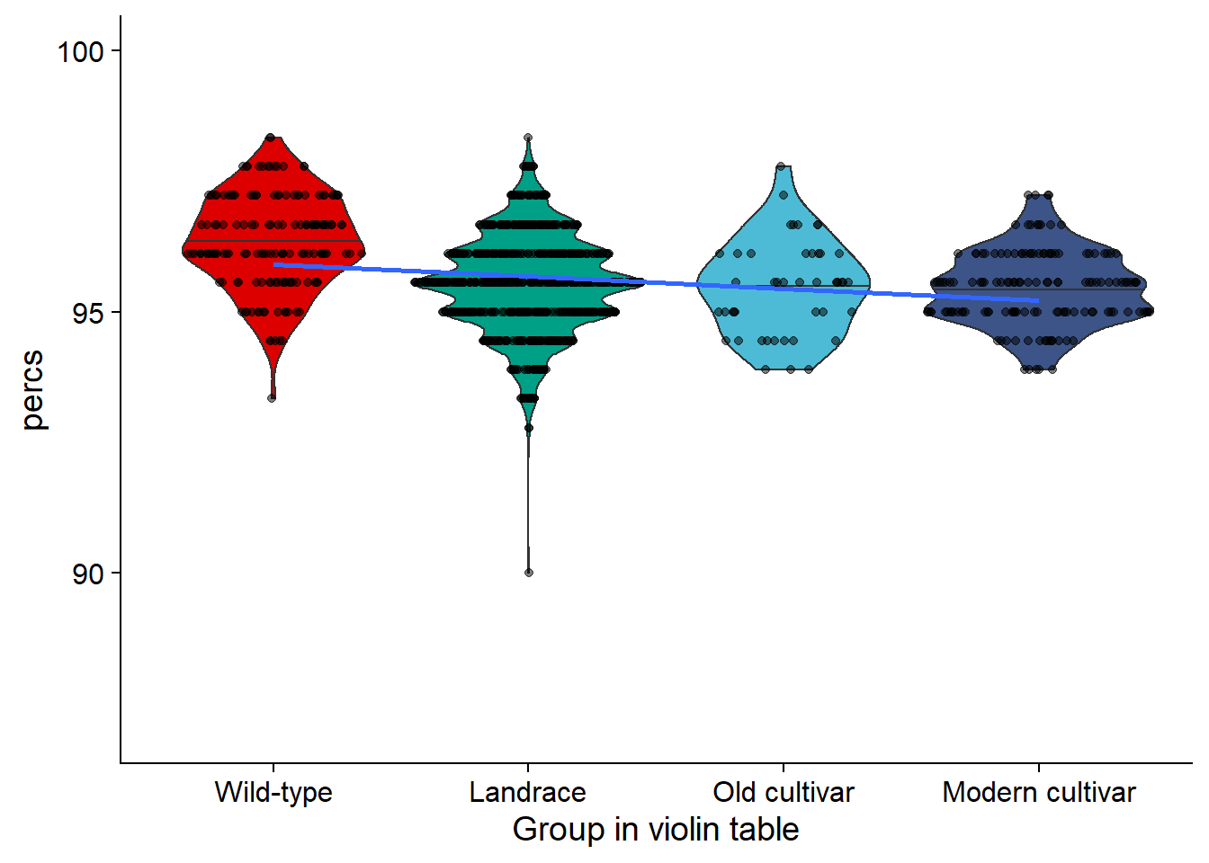

rlp_joined_groups %>% filter(`Group in violin table` != 'NA') %>% 
  ggplot(aes(y=percs, x=`Group in violin table`, fill=`Group in violin table`)) + 
  geom_jitter() +
  #geom_sina(alpha=0.5) +
  scale_fill_manual(values=col_list)+
  guides(fill = FALSE) +
  ylim(c(87, 100))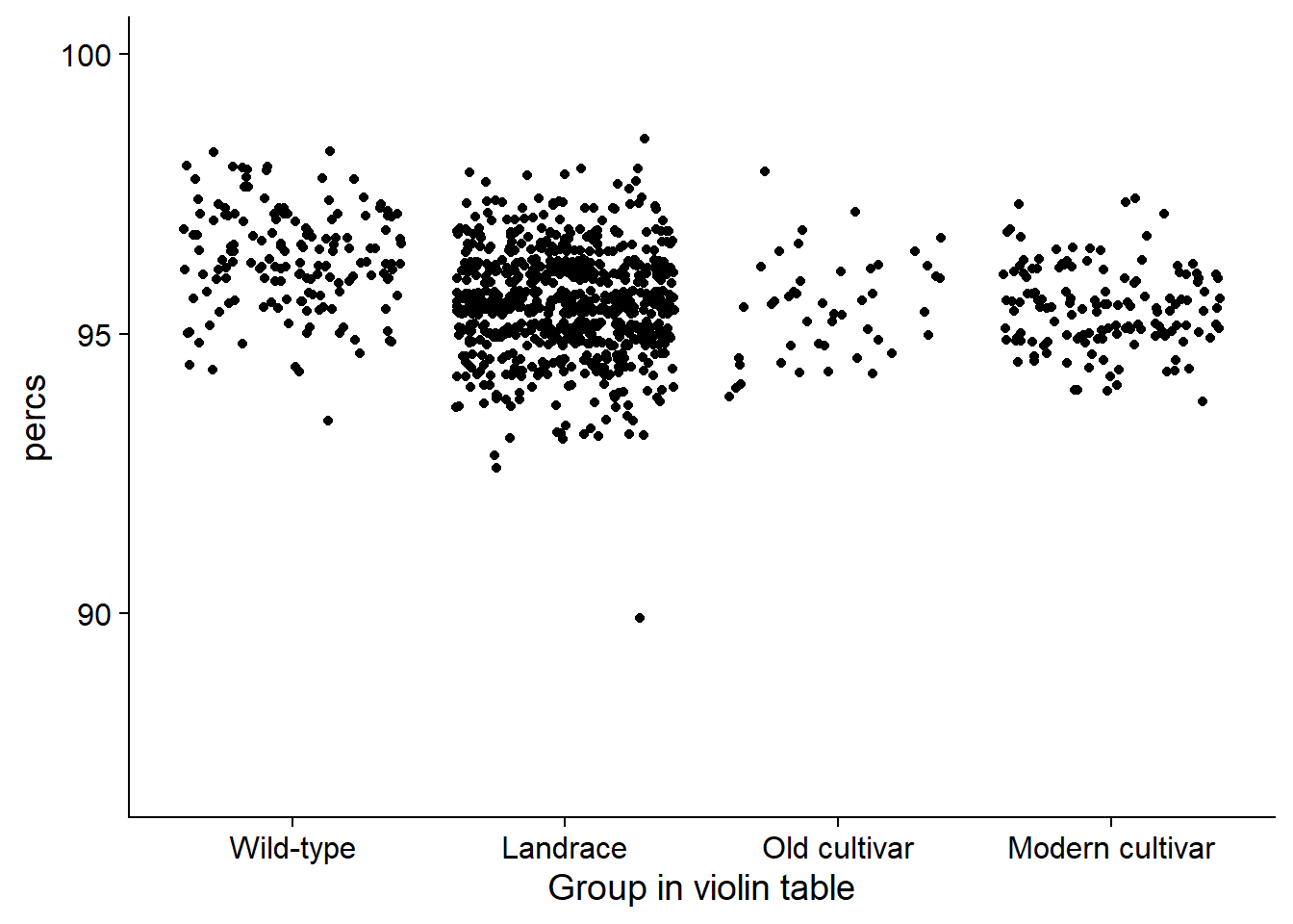

rlp_joined_groups %>% filter(!is.na(`PI-ID`)) %>% 
  group_by(`Group in violin table`) %>% 
  summarise(min_perc = min(percs),
            max_perc = max(percs),
            mean_perc = mean(percs),
            median_perc = median(percs),
            std_perc = sd(percs)) %>% 
  knitr::kable()

Group in violin table	min_perc	max_perc	mean_perc	median_perc	std_perc
Wild-type	93.33333	98.33333	96.34112	96.11111	0.8985510
Landrace	90.00000	98.33333	95.53711	95.55556	0.9230701
Old cultivar	93.88889	97.77778	95.45894	95.55556	0.9019439
Modern cultivar	93.88889	97.22222	95.44678	95.55556	0.7169931

Plotting together

nbs_vio + rlk_vio + rlp_vio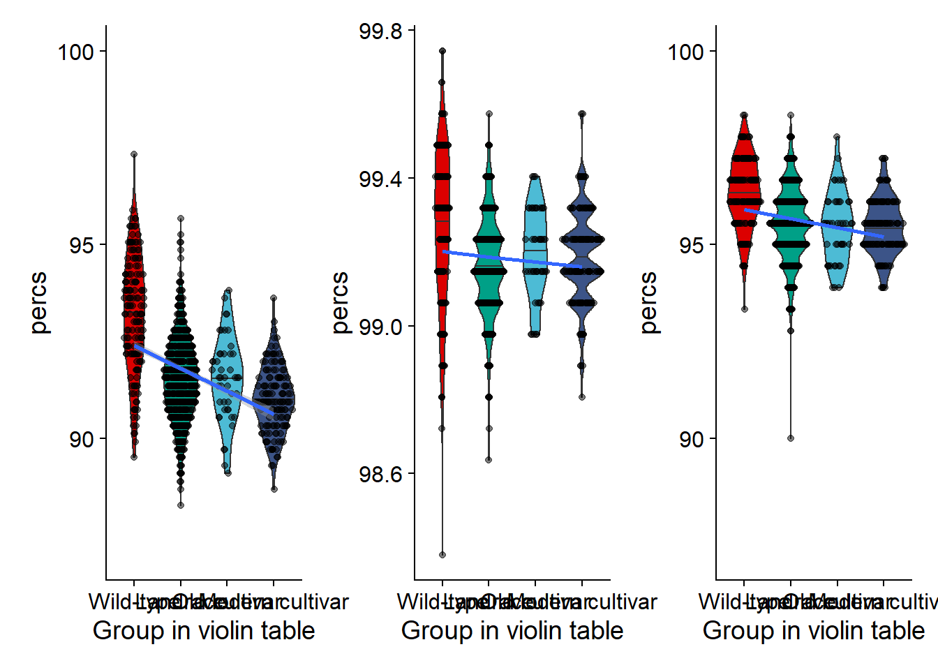

Stats - Dabayes

I want to know whether the groups are statistically significantly different. First let’s use dabestr

NBS

Let’s run dabestr first:

nbs_multi.two.group.unpaired <- 
  nbs_joined_groups %>% filter(!is.na(`PI-ID`)) %>% 
  dabest(`Group in violin table`, percs, 
         idx = list(c("Wild-type", "Landrace"),
                    c('Old cultivar', 'Modern cultivar')),
         paired = FALSE)
nbs_multi.two.group.unpaired

dabestr (Data Analysis with Bootstrap Estimation in R) v0.3.0
=============================================================

Good morning!
The current time is 11:04 AM on Friday December 11, 2020.

Dataset    :  .
The first five rows are:
# A tibble: 5 x 4
  names  percs `PI-ID`  `Group in violin table`
  <chr>  <dbl> <chr>    <fct>                  
1 AB-01   91.6 PI458020 Landrace               
2 AB-02   93.4 PI603713 Landrace               
3 DT2000  92.0 PI635999 Modern cultivar        
4 For     92.2 PI548645 Modern cultivar        
5 HN001   92.2 PI518664 Modern cultivar        

X Variable :  Group in violin table
Y Variable :  percs

Effect sizes(s) will be computed for:
  1. Landrace minus Wild-type
  2. Modern cultivar minus Old cultivar

nbs_multi.two.group.unpaired.meandiff <- mean_diff(nbs_multi.two.group.unpaired)
nbs_multi.two.group.unpaired.meandiff

dabestr (Data Analysis with Bootstrap Estimation in R) v0.3.0
=============================================================

Good morning!
The current time is 11:04 AM on Friday December 11, 2020.

Dataset    :  .
X Variable :  Group in violin table
Y Variable :  percs

Unpaired mean difference of Landrace (n = 723) minus Wild-type (n = 157)
 -1.66 [95CI  -1.9; -1.41]

Unpaired mean difference of Modern cultivar (n = 143) minus Old cultivar (n = 46)
 -0.526 [95CI  -0.875; -0.2]


5000 bootstrap resamples.
All confidence intervals are bias-corrected and accelerated.

plot(nbs_multi.two.group.unpaired.meandiff, color.column=`Group in violin table`,
     rawplot.ylabel = 'Presence (%)', show.legend=FALSE)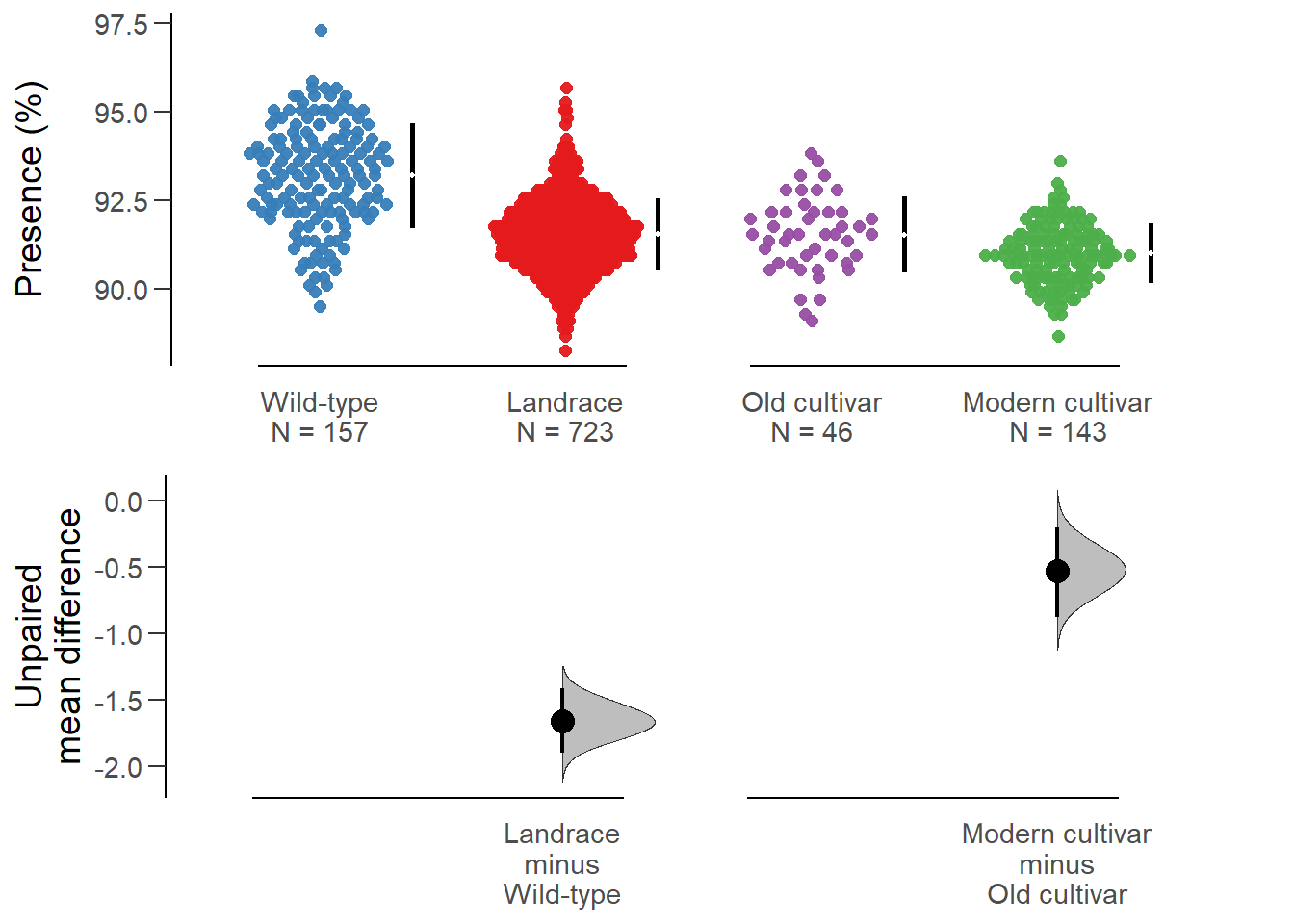

RLK

rlk_multi.two.group.unpaired <- 
  rlk_joined_groups %>% filter(!is.na(`PI-ID`)) %>% 
  dabest(`Group in violin table`, percs, 
         idx = list(c("Wild-type", "Landrace"),
                    c('Old cultivar', 'Modern cultivar')),
         paired = FALSE)
rlk_multi.two.group.unpaired

dabestr (Data Analysis with Bootstrap Estimation in R) v0.3.0
=============================================================

Good morning!
The current time is 11:04 AM on Friday December 11, 2020.

Dataset    :  .
The first five rows are:
# A tibble: 5 x 4
  names  percs `PI-ID`  `Group in violin table`
  <chr>  <dbl> <chr>    <fct>                  
1 AB-01   99.5 PI458020 Landrace               
2 AB-02   99.1 PI603713 Landrace               
3 DT2000  99.3 PI635999 Modern cultivar        
4 For     99.1 PI548645 Modern cultivar        
5 HN001   99.1 PI518664 Modern cultivar        

X Variable :  Group in violin table
Y Variable :  percs

Effect sizes(s) will be computed for:
  1. Landrace minus Wild-type
  2. Modern cultivar minus Old cultivar

rlk_multi.two.group.unpaired.meandiff <- mean_diff(rlk_multi.two.group.unpaired)
rlk_multi.two.group.unpaired.meandiff

dabestr (Data Analysis with Bootstrap Estimation in R) v0.3.0
=============================================================

Good morning!
The current time is 11:04 AM on Friday December 11, 2020.

Dataset    :  .
X Variable :  Group in violin table
Y Variable :  percs

Unpaired mean difference of Landrace (n = 723) minus Wild-type (n = 157)
 -0.0971 [95CI  -0.132; -0.0611]

Unpaired mean difference of Modern cultivar (n = 143) minus Old cultivar (n = 46)
 -0.00831 [95CI  -0.0479; 0.0308]


5000 bootstrap resamples.
All confidence intervals are bias-corrected and accelerated.

plot(rlk_multi.two.group.unpaired.meandiff, color.column=`Group in violin table`,
     rawplot.ylabel = 'Presence (%)', show.legend=FALSE)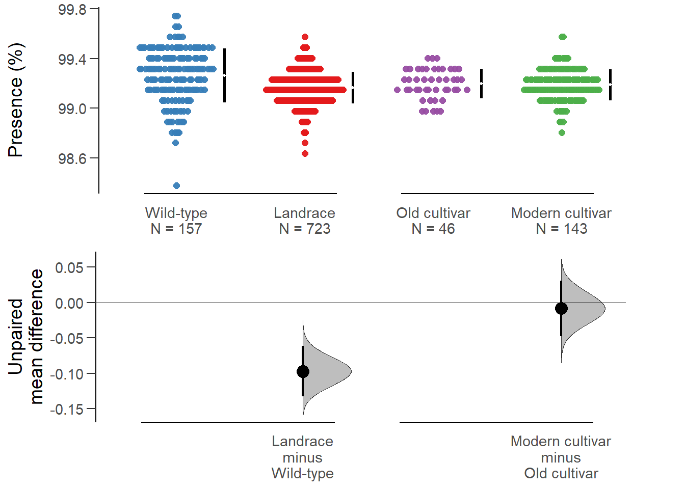

No difference between old and modern cultivars!

RLP

rlp_multi.two.group.unpaired <- 
  rlp_joined_groups %>% filter(!is.na(`PI-ID`)) %>% 
  dabest(`Group in violin table`, percs, 
         idx = list(c("Wild-type", "Landrace"),
                    c('Old cultivar', 'Modern cultivar')),
         paired = FALSE)
rlp_multi.two.group.unpaired

dabestr (Data Analysis with Bootstrap Estimation in R) v0.3.0
=============================================================

Good morning!
The current time is 11:04 AM on Friday December 11, 2020.

Dataset    :  .
The first five rows are:
# A tibble: 5 x 4
  names  percs `PI-ID`  `Group in violin table`
  <chr>  <dbl> <chr>    <fct>                  
1 AB-01   95   PI458020 Landrace               
2 AB-02   95.6 PI603713 Landrace               
3 DT2000  95   PI635999 Modern cultivar        
4 For     95   PI548645 Modern cultivar        
5 HN001   95.6 PI518664 Modern cultivar        

X Variable :  Group in violin table
Y Variable :  percs

Effect sizes(s) will be computed for:
  1. Landrace minus Wild-type
  2. Modern cultivar minus Old cultivar

rlp_multi.two.group.unpaired.meandiff <- mean_diff(rlp_multi.two.group.unpaired)
rlp_multi.two.group.unpaired.meandiff

dabestr (Data Analysis with Bootstrap Estimation in R) v0.3.0
=============================================================

Good morning!
The current time is 11:04 AM on Friday December 11, 2020.

Dataset    :  .
X Variable :  Group in violin table
Y Variable :  percs

Unpaired mean difference of Landrace (n = 723) minus Wild-type (n = 157)
 -0.804 [95CI  -0.965; -0.651]

Unpaired mean difference of Modern cultivar (n = 143) minus Old cultivar (n = 46)
 -0.0122 [95CI  -0.294; 0.265]


5000 bootstrap resamples.
All confidence intervals are bias-corrected and accelerated.

plot(rlp_multi.two.group.unpaired.meandiff, color.column=`Group in violin table`,
     rawplot.ylabel = 'Presence (%)', show.legend=FALSE)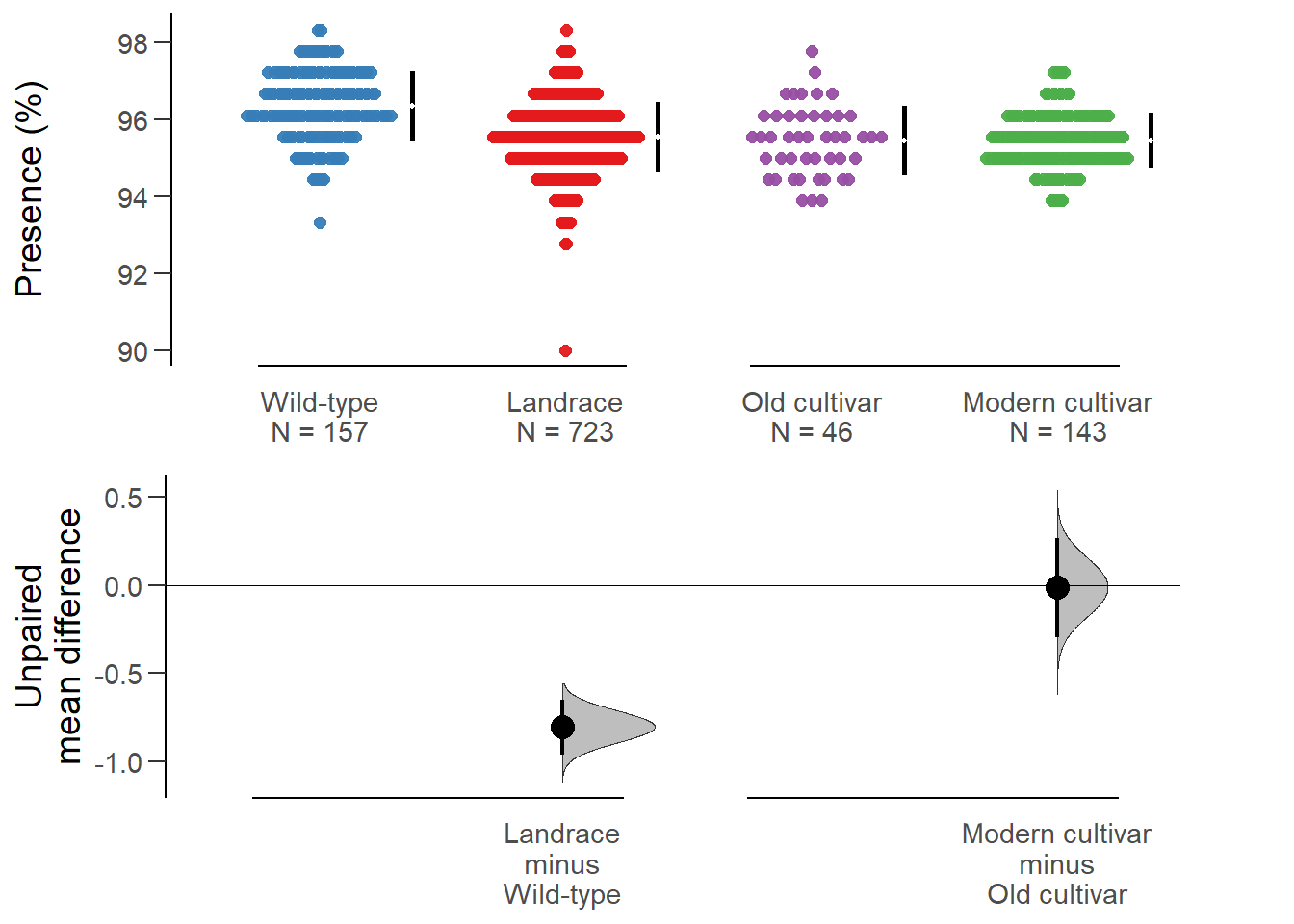

Again, no difference between old and modern cultivars!

Stats - classic t-test

NBS

nbs_joined_groups %>% 
  filter( !is.na(`PI-ID`) ) %>%
    ggplot(aes(x=`Group in violin table`, y = percs,
               fill = `Group in violin table`)) + 
  geom_boxplot() +
  scale_fill_manual(values = col_list) + 
  theme_minimal_hgrid() +
  theme(axis.text.x = element_text(size=12),
        axis.text.y = element_text(size=12)) +
  geom_signif(comparisons = list(c('Wild-type', 'Landrace'),
                                 c('Old cultivar', 'Modern cultivar')), 
              map_signif_level = T) +
  guides(fill=FALSE)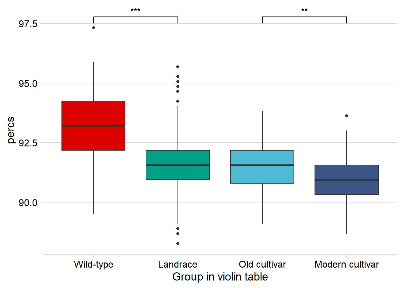

RLP

rlp_joined_groups %>% 
  filter( !is.na(`PI-ID`) ) %>%
    ggplot(aes(x=`Group in violin table`, y = percs,
               fill = `Group in violin table`)) + 
  geom_boxplot() +
  scale_fill_manual(values = col_list) + 
  theme_minimal_hgrid() +
  theme(axis.text.x = element_text(size=12),
        axis.text.y = element_text(size=12)) +
  geom_signif(comparisons = list(c('Wild-type', 'Landrace'),
                                 c('Old cultivar', 'Modern cultivar')), 
              map_signif_level = T) +
  guides(fill=FALSE)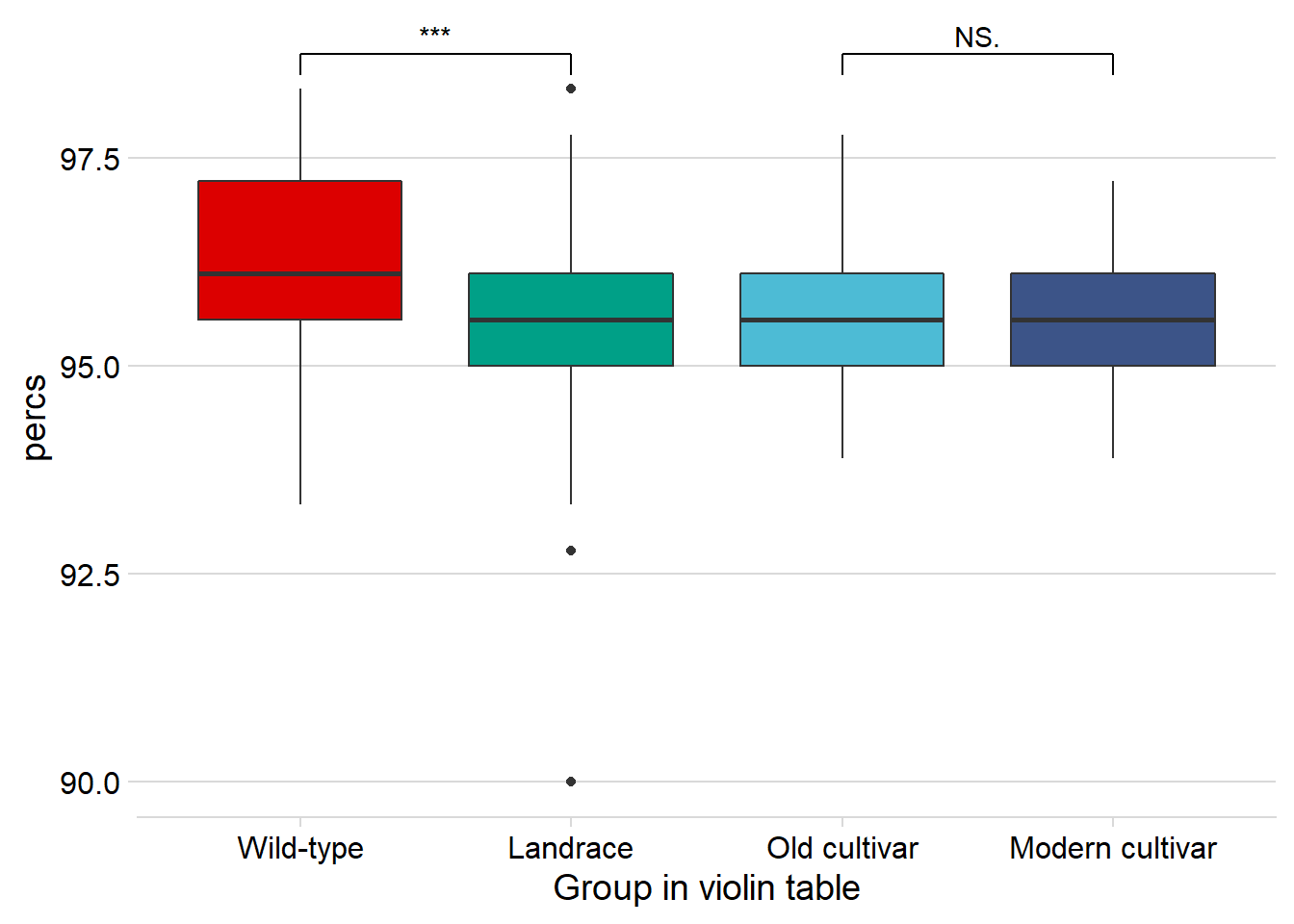

RLK

rlk_joined_groups %>% 
  filter( !is.na(`PI-ID`) ) %>%
    ggplot(aes(x=`Group in violin table`, y = percs,
               fill = `Group in violin table`)) + 
  geom_boxplot() +
  scale_fill_manual(values = col_list) + 
  theme_minimal_hgrid() +
  theme(axis.text.x = element_text(size=12),
        axis.text.y = element_text(size=12)) +
  geom_signif(comparisons = list(c('Wild-type', 'Landrace'),
                                 c('Old cultivar', 'Modern cultivar')), 
              map_signif_level = T) +
  guides(fill=FALSE)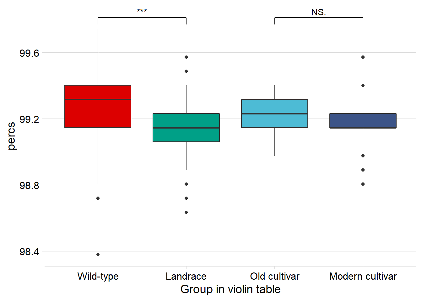

sessionInfo()

R version 3.6.3 (2020-02-29)
Platform: x86_64-w64-mingw32/x64 (64-bit)
Running under: Windows 10 x64 (build 17134)

Matrix products: default

locale:
[1] LC_COLLATE=English_Australia.1252  LC_CTYPE=English_Australia.1252   
[3] LC_MONETARY=English_Australia.1252 LC_NUMERIC=C                      
[5] LC_TIME=English_Australia.1252    

attached base packages:
[1] stats     graphics  grDevices utils     datasets  methods   base     

other attached packages:
 [1] ggforce_0.3.1        ggsignif_0.6.0       cowplot_1.0.0       
 [4] dabestr_0.3.0        magrittr_1.5         ggsci_2.9           
 [7] patchwork_1.0.0      forcats_0.5.0        stringr_1.4.0       
[10] dplyr_1.0.0          purrr_0.3.4          readr_1.3.1         
[13] tidyr_1.1.0          tibble_3.0.2         ggplot2_3.3.2       
[16] tidyverse_1.3.0      workflowr_1.6.2.9000

loaded via a namespace (and not attached):
 [1] nlme_3.1-148       fs_1.5.0.9000      lubridate_1.7.9    RColorBrewer_1.1-2
 [5] httr_1.4.2         rprojroot_1.3-2    tools_3.6.3        backports_1.1.10  
 [9] utf8_1.1.4         R6_2.4.1           vipor_0.4.5        DBI_1.1.0         
[13] mgcv_1.8-31        colorspace_1.4-1   withr_2.2.0        tidyselect_1.1.0  
[17] processx_3.4.4     compiler_3.6.3     git2r_0.27.1       cli_2.0.2         
[21] rvest_0.3.5        xml2_1.3.2         labeling_0.3       scales_1.1.1      
[25] callr_3.4.4        digest_0.6.25      rmarkdown_2.3      pkgconfig_2.0.3   
[29] htmltools_0.5.0    dbplyr_1.4.4       highr_0.8          rlang_0.4.7       
[33] readxl_1.3.1       rstudioapi_0.11    farver_2.0.3       generics_0.0.2    
[37] jsonlite_1.7.1     Matrix_1.2-18      Rcpp_1.0.5         ggbeeswarm_0.6.0  
[41] munsell_0.5.0      fansi_0.4.1        lifecycle_0.2.0    stringi_1.5.3     
[45] whisker_0.4        yaml_2.2.1         MASS_7.3-51.6      plyr_1.8.6        
[49] grid_3.6.3         blob_1.2.1         promises_1.1.1     crayon_1.3.4      
[53] lattice_0.20-41    haven_2.3.1        splines_3.6.3      hms_0.5.3         
[57] knitr_1.29         ps_1.3.4           pillar_1.4.4       boot_1.3-25       
[61] reprex_0.3.0       glue_1.4.2         evaluate_0.14      getPass_0.2-2     
[65] modelr_0.1.8       vctrs_0.3.1        tweenr_1.0.1       httpuv_1.5.4      
[69] cellranger_1.1.0   gtable_0.3.0       polyclip_1.10-0    assertthat_0.2.1  
[73] xfun_0.17          broom_0.5.6        later_1.1.0.1      beeswarm_0.2.3    
[77] ellipsis_0.3.1

first-analysis

Philipp Bayer

2020-09-17

Introduction

NBS part

RLK part

RLP part

Plotting together

Stats - Dabayes

NBS

RLK

RLP

Stats - classic t-test

NBS

RLP

RLK